Chapter 15 Computations on Iteration Spaces
15.1 Introduction
This chapter consists of two independent parts. The first deals with programs involving indexed data sets such as dense arrays and indexed computations such as loops. Our position is that high-level mathematical equations are the most natural way to express a large class of such computations, and furthermore, such equations are amenable to powerful static analyses that would enable a compiler to derive very efficient code, possibly significantly better than what a human would write. We illustrate this by describing a simple equational language and its semantic foundations and by illustrating the analyses we can perform, including one that allows the compiler to reduce the degree of the polynomial complexity of the algorithm embodied in the program.
The second part of this chapter deals with tiling, an important program reordering transformation applicable to imperative loop programs. It can be used for many different purposes. On sequential machines tiling can improve the locality of programs by exploiting reuse, so that the caches are used more effectively. On parallel machines it can also be used to improve the granularity of programs so that the communication and computation "units" are balanced.
We describe the tiling transformation, an optimization problem for selecting tile sizes, and how to generate tiled code for codes with regular or affine dependences between loop iterations. We also discuss approaches for reordering iterations, parallelizing loops, and tiling sparse computations that have irregular dependences.
15.2 The -Polyhedral Model and Some Static Analyses
It has been widely accepted that the single most important attribute of a programming language is programmer productivity. Moreover, the shift to multi-core consumer systems, with the number of cores expected to double every year, necessitates the shift to parallel programs. This emphasizes the need for productivity even further, since parallel programming is substantially harder than writing unithreadedcode. Even the field of high-end computing, typically focused exclusively on performance, is becoming concerned with the unacceptably high cost per megaflop of current high-end systems resulting from the required programming expertise. The current initiative is to increase programmability, portability, and robustness. DARPA's High Productivity Computing Systems (HPCSs) program aims to reevaluate and redesign the computing paradigms for high-performance applications from architectural models to programming abstractions.
We focus on compute- and data-intensive computations. Many data-parallel models and languages have been developed for the analysis and transformation of such computations. These models essentially abstract programs through (a) variables representing collections of values, (b) pointwise operations on the elements in the collections, and (c) collection-level operations. The parallelism may either be specified explicitly or derived automatically by the compiler. Parallelism detection involves analyzing the dependence between computations. Computations that are independent may be executed in parallel.
We present high-level mathematical equations to describe data-parallel computations succinctly and precisely. Equations describe the kernels of many applications. Moreover, most scientific and mathematical computations, for example, matrix multiplication, LU-decomposition, Cholesky factorization, Kalman filtering, as well as many algorithms arising in RNA secondary structure prediction, dynamic programming, and so on, are naturally expressed as equations.
It is also widely known that high-level programming languages increase programmer productivity and software life cycles. The cost of this convenience comes in the form of a performance penalty compared to lower-level implementations. With the subsequent improvement of compilation technology to accommodate these higher-level constructs, this performance gap narrows. For example, most programmers never use assembly language today. As a compilation challenge, the advantages of programmability offered by equations need to be supplemented by performance. After our presentation of an equational language, we will present automatic analyses and transformations to reduce the asymptotic complexity and to parallelize our specifications. Finally, we will present a brief description of the generation of imperative code from optimized equational specifications. The efficiency of the generated imperative code is comparable to hand-optimized implementations.
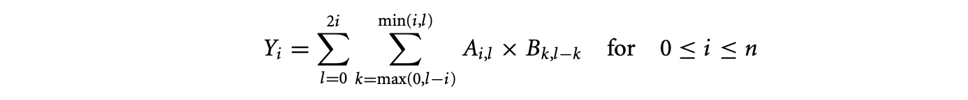
For an example of an equational specification and its automatic simplification, consider the following:
 Here, the variable is defined over a line segment, and the variables and , over a triangle and a square, respectively. These are the previously mentioned collections of values and are also called the domains of the respective variables. The dependence in the given computation is such that the value of at requires the value of at and the value of at for all valid values of and .
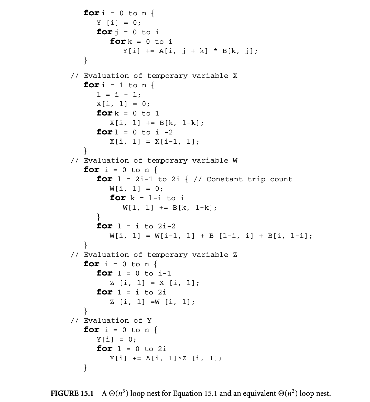
An imperative code segment that implements this equation is given in Figure 15.1. The triply nested loop (with linear bounds) indicates a asymptotic complexity for such an implementation. However, a implementation of Equation 15.1 exists and can be derived automatically. The code for this "simplified" specification is provided as well in Figure 15.1. The required sequence of transformations required to optimize the initial specification is given in Section 15.2.4. These transformations have been developed at the level of equations.
The equations presented so far have been of a very special form. It is primarily this special form that enables the development of sophisticated analyses and transformations. Analyses on general equations are often impossible. The class of equations that we consider consist of (a) variables defined on -polyhedral domains with (b) dependences in the form of affine functions. These restrictions enable us to use linear algebraic theory and techniques. In Section 15.2.1, we present -polyhedra and associated mathematical objects in detail that abstract the iteration domains of loop nests. Then we show the advantages of manipulating -polyhedra over integer polyhedra. A language to express equations over -polyhedral domains is presented in Section 15.2.3. The latter half of this section presents transformations to automatically simplify and parallelize equations. Finally, we provide a brief explanation of the transformations in the backend and code generation.
15.2.1 Mathematical Background1
Footnote 1: Parts of this section are adapted from [37], © 2007, Association for Computing Machinery, Inc., included by permission.
First, we review some mathematical background on matrices and decribe terminology. As a convention, we denote matrices with upper-case letters and vectors with lower-case. All our matrices and vectors have integer elements. We denote the identity matrix by . Syntactically, the different elements of a vector will be written as a list.
We use the following concepts and properties of matrices:
- The kernel of a matrix , written as , is the set of all vectors such that .
- The column (respectively row) rank of a matrix is the maximal number of linearly independent columns (respectively rows) of .
- A matrix is unimodular if it is square and its determinant is either or .
Figure 15: A loop nest for Equation 15.1 and an equivalent loop nest.
- Two matrices and are said to be column equivalent or right equivalent if there exists a unimodular matrix such that .
- A unique representative element in each set of matrices that are column equivalent is the one in Hermite normal form (HNF).
Definition 15.1:
An matrix with column rank is in HNF if:
-
For columns ,, , the first nonzero element is positive and is below the first positive element for the previous column.

-
In the first columns, all elements above the first positive element are zero.

-
The first positive entry in columns ,, is the maximal entry on its row. All elements are nonnegative in this row.

-
Columns are zero columns.

A template of a matrix in HNF is provided above. In the template, denotes the maximum element in the corresponding row, denotes elements that are not the maximum element, and denotes any integer. Both and are nonnegative elements.
For every matrix , there exists a unique matrix that is in HNF and column equivalent to , that is, there exists a unimodular matrix such that . Note that the provided definition of the HNF does not require the matrix to have full row rank.
15.2.1 Integer Polyhedra
An integer polyhedron, , is a subset of that can be defined by a finite number of affine inequalities (also called affine constraints or just constraints when there is no ambiguity) with integer coefficients. We follow the convention that the affine constraint is given as , where . The integer polyhedron, , satisfying the set of constraints , is often written as , where is an matrix and is a -vector.
Example 15.1:
Consider the equation
 The domains of the variables , , and are, respectively, the sets , , and . These sets are polyhedra, and deriving the aforementioned representation simply requires us to obtain, through elementary algebra, all affine constraints of the correct form, yielding , , and , respectively. Nevertheless, these are less intuitive, and in our presentation, we will not conform to the formalities of representation.
A subtle point to note here is that elements of polyhedral sets are tuples of integers. The index variables , , , and are simply place holders and can be substituted by other unused names. The domain of can also be specified by the set .
We shall use the following properties and notation of integer polyhedra and affine constraints:
- For any two coefficients and , where , and , is said to be a convex combination of and . If and are two iteration points in an integer polyhedron, , then any convex combination of and that has all integer elements is also in .
- The constraint of is said to be saturated iff.
- The lineality space of is defined as the linear part of the largest affine subspace contained in . It is given by .
- The context of is defined as the linear part of the smallest affine subspace that contains . If the saturated constraints in are the rows of , then the context of is .
15.2.1.1 Parameterized Integer Polyhedra
Recall Equation 15.1. The domain of is given by the set . Intuitively, the variable is seen as a size parameter that indicates the problem instance under consideration. If we associate every iteration point in the domain of with the appropriate problem instance, the domain of would be described by the set . Thus, a parameterized integer polyhedron is an integer polyhedron where some indices are interpreted as size parameters.
An equivalence relation is defined on the set of iteration points in a parameterized polyhedron such that two iteration points are equivalent if they have identical values of size parameters. By this relation, a parameterized polyhedron is partitioned into a set of equivalence classes, each of which is identified by the vector of size parameters. Equivalence classes correspond to program instances and are, thus, called instances of the parameterized polyhedron. We identify size parameters by omitting them from the index list in the set notation of a domain.
15.2.1.2 Affine Images of Integer Polyhedra
An (standard) affine function, , is a function from iteration points to iteration points. It is of the form , where is an matrix and is an -vector.
Consider the integer polyhedron and the standard affine function given above. The image of under is of the form . These are the so-called linearly bound lattices (LBLs). The family of LBLs is a strict superset of the family of integer polyhedra. Clearly, every integer polyhedra is an LBL with and . However, for an example of an LBL that is not an integer polyhedron refer to Figure 15.2.

Figure 15.2: The LBL corresponding to the image of the polyhedron by the affine function does not contain the iteration point 8 but contains 7 and 9. Since 8 is a convex combination of 7 and 9, the set is not an integer polyhedron. Adapted from [37], © 2007, Association for Computing Machinery, Inc., included by permission.
15.2.1.3 Affine Lattices
Often, the domain over which an equation is specified, or the iteration space of a loop program, does not contain every integer point that satisfies a set of affine constraints.
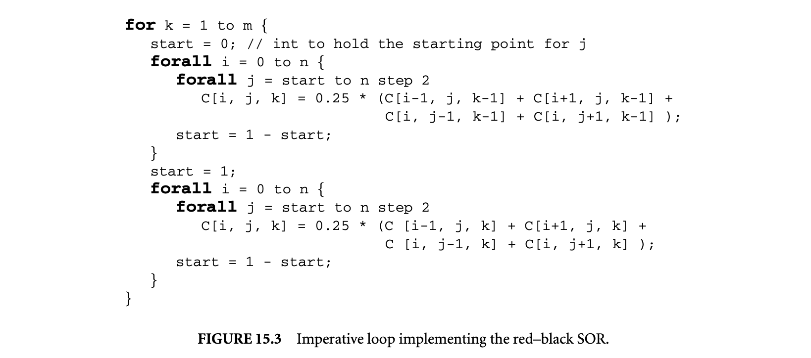
Example 15.2: Consider the red-black SOR for the iterative computation of partial differential equations. Iterations in the plane are divided into "red" points and "black" points, similar to the layout of squares in a chess board. First, black points (at even ) are computed using the four neighboring red points (at odd ), and then the red points are computed using its four neighboring black points. These two phases are repeated until convergence. Introducing an additional dimension, to denote the iterative application of the two phases, we get the following equation:
 where the domain of is , and are size parameters, and is given as input. The imperative loop nest that implements this equation is given in Figure 15.3.
We see that the first (respectively second) branch of the equation is not defined over all iteration points that satisfy a set of affine constraints, namely, , but over points that additionally satisfy (respectively ). This additional constraint in the first branch of the equation is satisfied precisely by the iteration points that can be expressed as an integer linear combination of the vectors . The vectors and are the generators of the lattice on which these iteration points lie.
The additional constraint in the second branch of the equation is satisfied precisely by iteration points that can be expressed as the following affine combination:
 Formally, the lattice generated by a matrix is the set of all integer linear combinations of the columns of . If the columns of a matrix are linearly independent, they constitute a basis of the generated lattice. The lattices generated by two-dimensionally identical matrices are equal iff the matrices are column equivalent. In general, the lattices generated by two arbitrary matrices are equal iff the submatrices corresponding to the nonzero columns in their HNF are equal.
As seen in the previous example, we need a generalization of the lattices generated by a matrix, additionally allowing offsets by constant vectors. These are called affine lattices. An affine lattice is a subset of of the form , where and are an matrix and -vector, respectively. We call the coordinates of the affine lattice.
The affine lattices and are equal iff the lattices generated by and are equal and for some constant vector . The latter requirement basically enforces that the offset of one lattice lies on the other lattice.
15.2.1.4 -Polyhedra
-polyhedron is the intersection of an integer polyhedron and an affine lattice. Recall the set of iteration points defined by either branch of the equation for the red-black SOR. As we saw above, these iteration points lie on an affine lattice in addition to satisfying a set of affine constraints. Thus, the set of these iteration points is precisely a -polyhedron. When the affine lattice is the canonical lattice, , a -polyhedron is also an integer polyhedron. We adopt the following representation for -polyhedra:
 where has full column rank, and the polyhedron has a context that is the universe, . is called the coordinate polyhedron of the -polyhedron. The -polyhedron for which has no columns has a coordinate polyhedron in .
We see that every -polyhedron is an LBL simply by observing that the representation for a -polyhedron is in the form of an affine image of an integer polyhedron. However, the LBL in Figure 15.2 is clearly not a -polyhedron. There does not exist any lattice with which we can intersect the integer polyhedron to get the set of iteration points of the LBL. Thus, the family of LBLs is a strict superset of the family of -polyhedra.
Our representation for -polyhedra as affine images of integer polyhedra is specialized through the restriction to and . We may interpret the -polyhedral representation in Equation 15.3 as follows. It is said to be based on the affine lattice given by . Iteration points of the -polyhedral domain are points of the affine lattice corresponding to valid coordinates. The set of valid coordinates is given by the coordinate polyhedron.
15.2.1.4.1 Parameterized -Polyhedra
parameterized -polyhedron is a -polyhedron where some rows of its corresponding affine lattice are interpreted as size parameters. An equivalence relation is defined on the set of iteration points in a parameterized -polyhedron such that two iteration points are equivalent if they have identical value of size parameters. By this relation, a parameterized -polyhedron is partitioned into a set of equivalence classes, each of which is identified by the vector of size parameters. Equivalence classes correspond to program instances and are, thus, called instances of the parameterized -polyhedron.
For the sake of explanation, and without loss of generality, we may impose that the rows that denote size parameters are before all non-parameter rows. The equivalent -polyhedron based on the HNF of such a lattice has the important property that all points of the coordinate polyhedron with identical values of the first few indices belong to the same instance of the parameterized -polyhedron.
Example 15.3
Consider the -polyhedron given by the intersection of the polyhedron and the lattice .1 It may be written as

For both the polyhedron and the affine lattice, the specification of the coordinate space is redundant. It can be derived from the number of indices and is therefore dropped for the sake of brevity.
Now, suppose the first index, , in the polyhedron is the size parameter. As a result, the first row in the lattice corresponding to the -polyhedron is the size parameter. The HNF of this lattice is . The equivalent -polyhedron is

The iterations of this -polyhedron belong to the same program instance iff they have the same coordinate index . Note that valid values of the parameter row trivially have a one-to-one correspondence with values of , identity being the required bijection. In the general case, however, this is not the case. Nevertheless, the required property remains invariant. For example, consider the following -polyhedron with the first two rows considered as size parameters:
 Here, valid values of the parameter rows have a one-to-one correspondence with the values of and , but it is impossible to obtain identity as the required bijection.
15.2.1.5 Affine Lattice Functions
Affine lattice functions are of the form , where has full column rank. Such functions provide a mapping from the iteration to the iteration . We have imposed that have full column rank to guarantee that be a function and not a relation, mapping any point in its domain to a unique point in its range. All standard affine functions are also affine lattice functions.
The mathematical objects introduced here are used to abstract the iteration domains and dependences between computations. In the next two sections, we will show the advantages of manipulating equations with -polyhedral domains instead of polyhedral domains and present a language for the specification of such equations.
15.2.2 The -Polyhedral Model
We will now develop the -polyhedral model that enables the specification, analysis, and transformation of equations described over -polyhedral domains. It has its origins in the polyhedral model that has been developed for over a quarter century. The polyhedral model has been used in a variety of contexts, namely, automatic parallelization of loop programs, locality, hardware generation, verification, and, more recently, automatic reduction of asymptotic computational complexity. However, the prime limitation of the polyhedral model lay in its requirement for dense iteration domains. This motivated the extension to -polyhedral domains. As we have seen in the red-black SOR, -polyhedral domains describe the iterations of a regular loop with non-unit stride.
In addition to allowing more general specifications, the -polyhedral model enables more sophisticated analyses and transformations by providing greater information in the specifications, namely, pertaining to lattices. The example below demonstrates the advantages of manipulating -polyhedral domains. The variable is defined over the domain .2
Code fragments in this section are adapted from [37], © 2007, Association for Computing Machinery, Inc., included by permission.
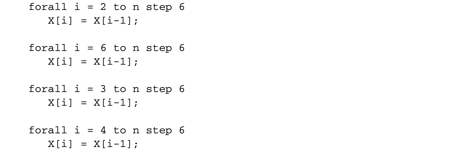
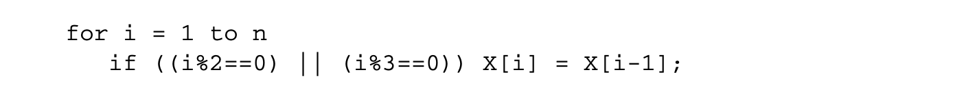 In the loop, only iteration points that are a multiple of 2 or 3 execute the statement . The iteration at may be excluded from the loop nest. Generalizing, any iteration that can be written in the form may be excluded from the loop nest. The same argument applies to iterations that can be written in the form . As result of these "holes," all iterations at may be executed in parallel at the first time step. The iterations at may also be executed in parallel at the first time step. At the next time step, we may execute iterations at and finally at iterations . The length of the longest dependence chain is 3. Thus, the loop nest can be parallelized to execute in constant time as follows:
 However, our derivation of parallel code requires to manipulate -polyhedral domains. A polyhedral approximation of the problem would be unable to result in such a parallelization.
Finally, the -polyhedral model allows specifications with a more general dependence pattern than the specifications in the polyhedral model. Consider the following equation that cannot be expressed in the polyhedral model.
 where and the corresponding loop is
 This program exhibits a dependence pattern that is richer than the affine dependences of the polyhedral model. In other words, it is impossible to write an equivalent program in the polyhedral model, that is, without the use of the mod operator or non-unit stride loops, that can perform the required computation. One may consider replacing the variable with two variables and corresponding to the even and odd points of such that and . However, the definition of now requires the mod operator, because and .
Thus, the -polyhedral model is a strict generalization of the polyhedral model and enables more powerful optimizations.
15.2.3 Equational Language
In our presentation of the red-black SOR in Section 15.2.1.3, we studied the domains of the two branches of Equation 15.2. More specifically, these are the branches of the case expression in the right-hand side (rhs) of the equation. In general, our techniques require the analysis and transformation of the subexpressions that constitute the rhs of equations, treating expressions as first-class objects.
For example, consider the simplification of Equation 15.1. As written, the simplification transforms the accumulation expression in the rhs of the equation. However, one would expect the technique to be able to decrease the asymptotic complexity of the following equation as well.
 Generalizing, one would reasonably expect the existence of a technique to reduce the complexity of evaluation of the accumulation subexpression (), irrespective of its "level." This motivates a homogeneous treatment of the subexpression at any level. At the lowest level of specification,a subexpression is a variable (or a constant) associated with a domain. Generalizing, we associate domains to arbitrary subexpressions.
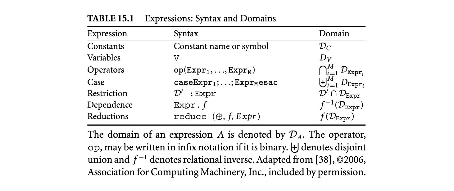 The treatment of expressions as first-class objects leads to the design of a functional language where programs are a finite list of (mutually recursive) equations of the form , where both Var and Expr denote mappings from their respective domains to a set of values (similar to multidimensional arrays). A variable is defined by at most one equation. Expressions are constructed by the rules given in Table 15.1, column 2. The domains of all variables are declared, the domains of constants are either declared or defined over by default, and the domains of expressions are derived by the rules given in Table 15.1, column 3. The function specified in a dependence expression is called the dependence function (or simply a dependence), and the function specified in a reduction is called the projection function (or simply a projection).
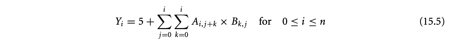
In this language, Equation 15.5 would be a syntactically sugared version of the following concrete problem.
 In the equation above, 5 is a constant expression defined over and Y, A, and B are variables. In addition to the equation, the domains of Y, A, and B would be declared as the sets , , and , respectively. The reduction expression is the accumulation in Equation 15.5. Summation is expressed by the reduction operator + (other possible reduction operators are *, max, min, or, and, etc.). The projection function (i,j,k->i) specifies that the accumulation is over the space spanned by and resulting in values in the one-dimensional space spanned by . A subtle and important detail is that the expression that is accumulated is defined over a domain in three-dimensional space spanned by , , and (this information is implicit in standard mathematical specifications as in Equation 15.5). This is an operator expression equal to the product of the value of at and at . In the space spanned by , , and , the required dependences on and are expressed through dependence expressions A.(i,j,k->i,j+k) and B.(i,j,k->k,j), respectively. The equation does not contain any case or restrict constructs. For an example of these two constructs, refer back to Equation 15.4. In our equational specification, the equation would be written as
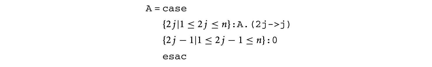 where the domains of and the constant are and , respectively. There are two branches of the case expression, each of which is a restriction expression. We have not provided domains of any of the subexpressions mentioned above for the sake of brevity. These can be computed using the rules given in Table 15.1, column 3.
15.2.3.1
Parts of this section are adapted from [38], © 2006, Association for Computing Machinery, Inc., included by permission.
At this point3, we intuitively understand the semantics of expressions. Here, we provide the formal semantics of expressions over their domains of definition. At the iteration point in its domain, the value of:
- A constant expression is the associated constant.
- A variable is either provided as input or given by an equation; in the latter case, it is the value, at , of the expression on its rhs.
- An operator expression is the result of applying on the values, at , of its expression arguments. is an arbitrary, iteration-wise, single valued function.
- A case expression is the value at of that alternative, to whose domain belongs. Alternatives of a case expression are defined over disjoint domains to ensure that the case expression is not under- or overdefined.
- A restriction over is the value of at .
- The dependence expression is the value of at . For the affine lattice function , the value of the (sub)expression at equals the value of at .
- is the application of on the values of at all iteration points in that map to by . Since is an associative and commutative binary operator, we may choose any order of its application.
It is often convenient to have a variable defined either entirely as input or only by an equation. The former is called an input variable and the latter is a computed variable. So far, all our variables have been of these two kinds only. Computed variables are just names for valid expressions.
15.2.3.2 The Family of Domains
Variables (and expressions) are defined over -polyhedral domains. Let us study the compositional constructs in Table 15.1 to get a more precise understanding of the family of -polyhedral domains.
For compound expressions to be defined over the same family of domains as their subexpressions, the family should be closed under intersection (operator expressions, restrictions), union (case expression), and preimage (dependence expressions) and image (reduction expressions) by the family of functions. With closure, we mean that a (valid) domain operation on two elements of the family of domains should result in an element that also belongs to the family. For example, the family of integer polyhedra is closed under intersection but not under images, as demonstrated by the LBL in Figure 15.2. The family of integer polyhedra is closed under intersection since the intersection of two integer polyhedra that lie in the same dimensional space results in an integer polyhedron that satisfies the constraints of both the integer polyhedra.
In addition to intersection, union, and preimage and image by the family of functions, most analyses and transformations (e.g., simplification, code generation, etc.) require closure under the difference of two domains. With closure under the difference of domains, we may always transform any specification to have only input and computed variables.
The family of -polyhedral domains should be closed under the domain operations mentioned above. This constraint is unsatisfied if the elements of this family are -polyhedra. For example, the union of two -polyhedra is not a -polyhedron. Also, the LBL in Figure 15.2 shows that the image of a -polyhedron is not a -polyhedron. However, if the elements of the family of -polyhedral domains are unions of -polyhedra, then all the domain operations mentioned above maintain closure.
15.2.3.3 Parameterized Specifications
Extending the concept of parameterized -polyhedra, it is possible to parameterize the domains of variables and expressions with size parameters. This leads to parameterized equational specifications. Instances of the parameterized -polyhedra correspond to program instances.
 Every program instance in a parameterized specification is independent, so all functions should map consumer iterations to producer iterations within the same program instance.
15.2.3.4 Normalization
For most analyses and transformations (e.g., the simplification of reductions, scheduling, etc.), we need equations in a special normal form. Normalization is a transformation of an equational specification to obtain an equivalent specification containing only equations of the canonic forms or , where the expression is of the form
 and is a variable or a constant.
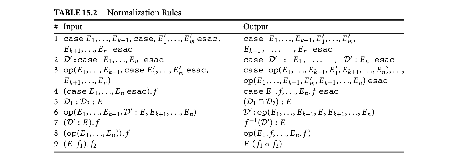
Such a normalization transformation4 first introduces an equation for every reduce expression, replacing its occurrence with the corresponding local variable. As a result, we get equations of the forms or , where the expression does not contain any reduce subexpressions. Subsequently, these expressions are processed by a rewrite engine to obtain equivalent expressions of the form specified in Equation 15.6. The rules for the rewrite engine are given in Table 15.2. Rules 1 to 4 "bubble" a single case expression to the outermost level, rules 5 to 7 then "bubble" a single restrict subexpression to the second level, rule 8 gets the operator to the penultimate level, and rule 9 is a dependence composition to obtain a single dependence at the innermost level.
and is a variable or a constant.
Such a normalization transformation4 first introduces an equation for every reduce expression, replacing its occurrence with the corresponding local variable. As a result, we get equations of the forms or , where the expression does not contain any reduce subexpressions. Subsequently, these expressions are processed by a rewrite engine to obtain equivalent expressions of the form specified in Equation 15.6. The rules for the rewrite engine are given in Table 15.2. Rules 1 to 4 "bubble" a single case expression to the outermost level, rules 5 to 7 then "bubble" a single restrict subexpression to the second level, rule 8 gets the operator to the penultimate level, and rule 9 is a dependence composition to obtain a single dependence at the innermost level.
More sophisticated normalization rules may be applied, expressing the interaction of reduce expressions with other subexpressions. However, these are unnecessary in the scope of this chapter.
The validity of these rules, in the context of obtaining a valid specification of the language, relies on the closure properties of the family of unions of -polyhedra.
15.2.4 Simplification of Reductions
Parts of this section are adapted from [38], © 2006, Association for Computing Machinery, Inc., included by permission.
We now provide a deeper study of reductions5. Reductions, commonly called accumulations, are the application of an associative and commutative operator to a collection of values to produce a collection of results.
Our use of equations was motivated by the simplification of asymptotic complexity of an equation involving reductions. We first present the required steps for the simplification. Then we will provide an intuitive explanation of the algorithm for simplification. For the sake of intuition, we use the standard mathematical notation for accumulations rather than the reduce expression.
Our initial specification was
 The loop nest corresponding to this equation has a complexity. The cubic complexity for this equation can also be directly deduced from the equational specification. Parameterized by , there are three independent7 indices within the summation. The following steps are involved in the derivation of the equivalent specification.
Footnote 7: With independent, we mean that there are no equalities between indices.
-
Introduce the index variable and replace every occurrence of with . This is a change of basis of the three-dimensional space containing the domain of the expression that is reduced.
The change in the order of summation is legal under our assumption that the reduction operator is associative and commutative.
-
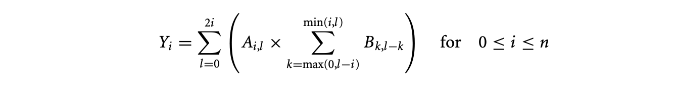
Distribute multiplication over the summation since is independent of , the index of the inner summation.
-
Introduce variable to hold the result of the inner summation
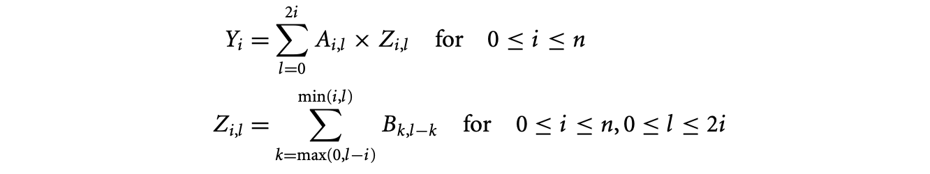 Note that the complexity of evaluating is now quadratic. However, we still have an equational specification that has cubic complexity (for the evaluation of ).
 -
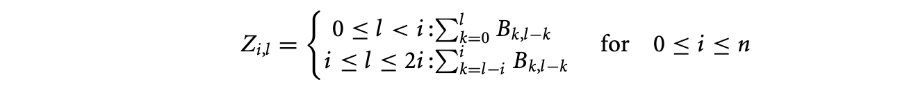
Separate the summation over to remove min and max operators in the equation for .
-
Introduce variables and for each branch of the equation defining .
 Both the equations given above have cubic complexity.
 -
Reuse. The complexity for the evaluation of can be decreased by identifying that the expression on the rhs is independent of . We may evaluate each result once (for instance, at a boundary) and then pipeline along as follows.
 The initialization takes quadratic time since there are a linear number of results to evaluate and each evaluation takes linear time. Then the pipelining of results over an area requires quadratic time. This decreases the overall complexity of evaluating to quadratic time.
 -
Scan detection. The simplification of occurs when we identify
 The values are, once again, initialized in quadratic time at a boundary (here, ). The scan takes constant time per iteration over an area and can be performed in quadratic time as well, thereby decreasing the complexity for the evaluation of to quadratic time.
 -
Summarizing, we have the following system of equations:
 These equations directly correspond to the optimized loop nest given in Figure 15. We have not optimized these equations or the loop nest any further for the sake for clarity, and moreso, because we only want to show an asymptotic decrease in complexity. However, a constant-fold improvement in the asymptotic complexity (as well as the memory requirement) can be obtained by eliminating the variable (or, alternatively, the two variables and ).
We now provide an intuitive explanation of the algorithm for simplification. Consider the reduction
 where is defined over the domain . The accumulation space of the above equation is characterized by . Any two points and that contribute to the same element of the result, , satisfy . To aid intuition, we may also write this reduction as
 is the "accumulation," using the operator, of the values of at all points that have the same image . Now, if has a distinct value at all points in its domain, they must all be computed, and no optimization is possible. However, consider the case where the expression exhibits reuse: its value is the same at many points in . Reuse is characterized by , the kernel of a many-to-one affine function, ;
 the value of at any two points in is the same if their difference belongs to . We can denote this reuse by , where is a variable with domain . In our language, this would be expressed by the dependence expression . The canonical equation that we analyze is
 Its nominal complexity is the cardinality of the domain of . The main idea behind our method is based on analyzing (a) , the domain of the expression inside the reduction, (b) its reuse space, and (c) the accumulation space.
15.2.4.1 Core Algorithm
Consider two adjacent instances of the answer variable, and along , where is a vector in the reuse space of . The set of values that contribute to and overlap. This would enable us to express in terms of . Of course, there would be residual accumulations on values outside the intersection that must be "added" or "subtracted" accordingly. We may repeat this for other values of along . The simplification results from replacing the original accumulation by a recurrence on and residual accumulations. For example, in the simple scan, , the expression inside the summation has reuse along . Taking , we get .
The geometric interpretation of the above reasoning is that we translate by a vector in the reuse space of . Let us call the translated domain . The intersection of and is precisely the domain of values, the accumulation over which can be avoided. Their differences account for the residual accumulations. In the simple scan explained above, the residual domain to be added is , and the domain to be subtracted is empty. The residual accumulations to be added or subtracted are determined only by and .
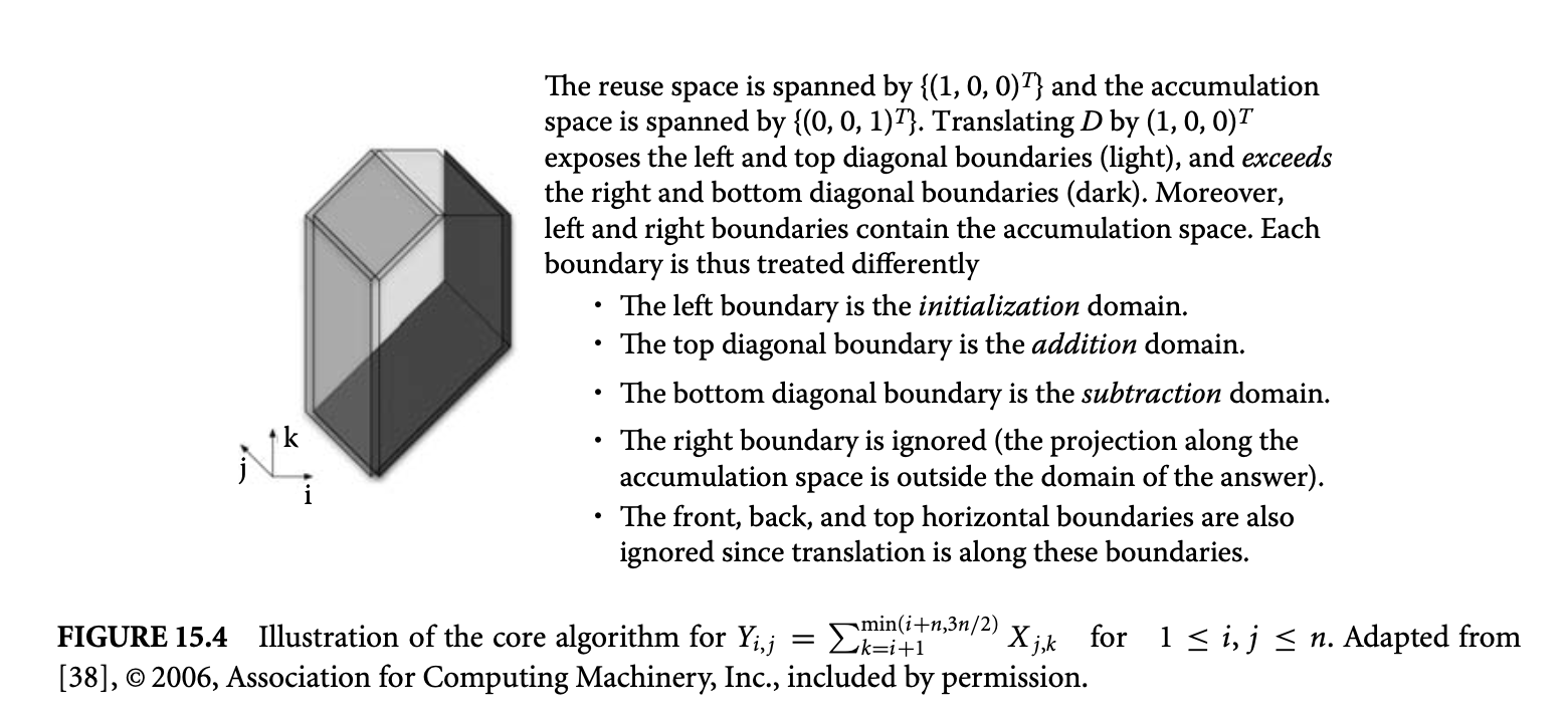
This leads to Algorithm 15.1 (also see Figure 15.4).
Algorithm 15.1 Intuition of the Core Algorithm6
Adapted from [38], © 2006, Association for Computing Machinery, Inc., included by permission.
- Choose , a vector in , along which the reuse of is to be exploited. In general, is multidimensional and therefore there may be infinitely many choices.
- Determine the domains , and corresponding to the domain of initialization, and the residual domains to subtract and to add, respectively. The choice of is made such that the cardinalities of these three domains are polynomials whose degree is strictly less than that for the original accumulation. This leads to simplification of the complexity.
Figure 15.4: Illustration of the core algorithm for for . Adapted from [38], © 2006, Association for Computing Machinery, Inc., included by permission.
- For these three domains, , , and , define the three expressions, , , and , consisting of the original expression , restricted to the appropriate subdomain.
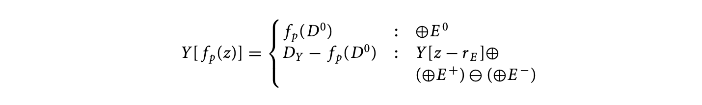
- Replace the original equation by the following recurrence:
- Apply steps 1 to 4 recursively on the residual reductions over , , or if they exhibit further reuse.
Note that Algorithm 15.1 assumes that the reduction operation admits an inverse; that is, "subtraction" is defined. If this is not the case, we need to impose constraints on the direction of reuse to exploit: essentially, we require that the domain is empty. This leads to a feasible space of exploitable reuse.
15.2.4.2 Multidimensional Reuse
When the reuse space as well as the accumulation space are multidimensional, there are some interesting interactions. Consider the equation for . It has two-dimensional reuse (in the plane), and the accumulation is also two-dimensional (in the plane). Note that the two subspaces intersect, and this means that in the direction, not only do all points have identical values, but they also all contribute to the same answer. From the bounds on the summation we see that there are exactly such values, so the inner summation is just , because multiplication is a higher-order operator for repeated addition of identical values (similar situations arise with other operators, e.g., power for multiplication, identity for the idempotent operator max, etc.). We have thus optimized the computation to . However, our original equation had two dimensions of reuse, and we may wonder whether further optimization is possible. In the new equation , the body is the product of two subexpressions, and . They both have one dimension of reuse, in the and directions, respectively, but their product does not. No further optimization is possible for this equation.
However, if we had first exploited reuse along , we would have obtained the simplified equation , initialized with . The residual reduction here is itself a scan, and we may recurse the algorithm to obtain and initialized with . Thus, our equation can be computed in linear time. This shows how the choice of reuse vectors to exploit, and their order, affects the final simplification.
15.2.4.3 Decomposition of Accumulation
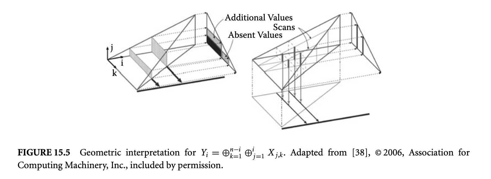
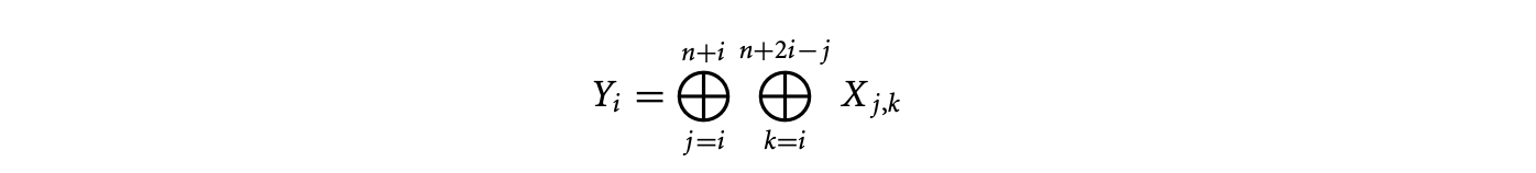
Consider the equation for . The one-dimensional reuse space is along , and is the two-dimensional accumulation space. The set of points that contribute to the th result lie in an rectangle of the two-dimensional input array . Comparing successive rectangles, we see that as the width decreases from one to the other, the height increases (Figure 15.5). If the operator does not have an inverse, it seems that we may not be able to simplify this equation. This is not true: we can see that for each we have an independent scan. The inner reduction is just a family of scans, which can be done in quadratic time with initialized with . The outer reduction just accumulates columns of , which is also quadratic.
What we did in this example was to decompose the original reduction that was along the space into two reductions, the inner along the space yielding partial answers along the plane and the outer that combined these partial answers along the space. Although the default choice of the decomposition -- the innermost accumulation direction -- of the space worked for this example, in general this is not the case. It is possible that the optimal solution may require a nonobvious decomposition, for instance,along some diagonal. We encourage the reader to simplify7 the following equation:
Solution: The inner reduction would map all points for which , for a given constant , to the same partial answer.
15.2.4.4 Distributivity and Accumulation Decomposition
Returning to the simplification of Equation 15.7, we see that the methods presented so far do not apply, since the body of the summation, , has no reuse. The expression has a distinct value at each point in the three-dimensional space spanned by , , and . However, the expression is composed of two subexpressions, which individually have reuse and are combined with the multiplication operator that distributes over the reduction operator, addition.
We may be able to distribute a subexpression outside a reduction if it has a constant value at all the points that map to the same answer. This was ensured by a change in basis of the three-dimensional space to , , and , followed by a decomposition to summations over and then . Values of were constant for different iterations of the accumulation over . After distribution, the body of the inner summation exhibited reuse that was exploited for the simplification of complexity.
15.2.5 Scheduling8
Adapted from [36] © 2007 IEEE, included by permission.
Scheduling is assigning an execution time to each computation so that precedence constraints are satisfied. It is one of the most important and widely studied problems. We present the scheduling analysis for programs in the -polyhedral model. The resultant schedule can be subsequently used to construct a space-time transformation leading to the generation of sequential or parallel code. The application of this schedule is made possible as a result of closure of the family of -polyhedral domains under image by the constructed transformation. We showed the advantages of scheduling programs in the -polyhedral model in Section 15.2.2. The general problem of scheduling programs with reductions is beyond the scope of this chapter. We will restrict our analysis to -polyhedral programs without reductions.
The steps involved in the scheduling analysis are (a) deriving precedence (causality) constraints for programs written in the -polyhedral model and (b) formulation of an integer linear program to obtain the schedule.
The precedence constraints between variables are derived from the reduced dependence graph (RDG). We will now provide some refinements of the RDG.
15.2.5.1 Basic and Refined RDG
Equations in the -polyhedral model can be defined over an infinite iteration domain. For any dependence analysis on an infinite graph, we need a compact representation. A directed multi-graph, the RDG precisely describes the dependences between iterations of variables. It is based on the normalized form of a specification and defined as follows:
- For every variable in the normalized specification, there is a vertex in the RDG labeled by the variable name and annotated by its domain. We will refer to vertices and variables interchangeably.
- For every dependence of the variable on , there is an edge from to , annotated by the corresponding dependence function. We will refer to edges and dependences interchangeably.
At a finer granularity, every branch of an equation in a normalized specification dictates the dependences between computations. A precise analysis requires that dependences be expressed separately for every branch. Again, for reasons of precision, we may express dependences of a variable separately for every -polyhedron in the -polyhedral domain of the corresponding branch of its equation. To enable these, we replace a variable by a set of new variables as elaborated below. Remember, our equations are of the form
 Let be written as a disjoint union of -polyhedra given by . The variable in the domain is replaced by a new variable, for instance, . Similarly, let be replaced by new variables given as . The dependence of in on is replaced by dependences from all on all . An edge from to may be omitted if there are no iterations in that map to (mathematically, if the preimage of by the dependence function does not intersect with ). A naive construction following these rules results in the basic reduced dependence graph.
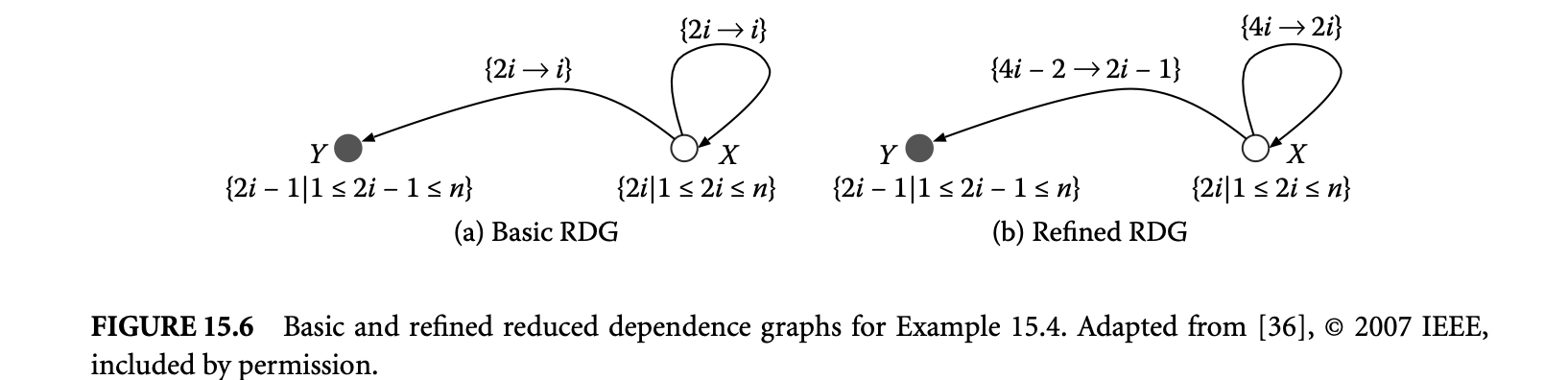
Figure 15.6a gives the basic RDG for Equation 15.4, which is repeated here for convenience.
 The domains of and the constant are and , respectively. Next, we will study a refinement on this RDG.
In the RDG for the generic equation given in Equation 15.10, let be a variable derived from and defined on , and let be a variable derived from defined on , where and are given as follows:
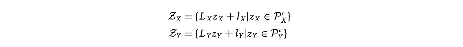
A dependence of the form is directed from to . at cannot be evaluated before at . The affine lattice may contain points that do not lie in the affine lattice . Similarly, the affine lattice may contain points that do not lie in the affine lattice . As a result, the dependence may be specified on a finer lattice than necessary and may safely be replaced by a dependence of the form , where
 where and are matrices and and are integer vectors. The refined RDG is a refinement of the basic RDG where every dependence has been replaced by a dependence satisfying Equation 15.11. Figure 15.6b gives the refined RDG for Equation 15.4.
15.2.5.2 Causality Constraints
Dependences between the different iterations of variables impose an ordering on their evaluation. A valid schedule of the evaluation of these iterations is the assignment of an execution time to each computation so that precedence (causality) constraints are satisfied.
Let and be two variables in the refined RDG defined on and , respectively. We seek to find schedules on and of the following form:
 where and are affine functions on and , respectively. Our motivation for such schedules is that all vectors and matrices are composed of integer scalars. If we seek schedules of the form , where is an affine function and is an iteration in the domain of a variable, then we may potentially assign execution times to "holes," or computations that do not exist.
We will now formulate causality constraints using the refined RDG. Consider dependences from to . All such dependences can be written as
 where and are matrices and and are vectors. The execution time for at should precede the execution time for at . With the nature of the schedules presented in Equation 15.12, our causality constraint becomes
 with the assumption that op is atomic and takes a single time step to evaluate.
From these constraints, we may derive an integer linear program to obtain schedules of the form , where is the lattice corresponding to the -polyhedron and is the affine function (composed of integer scalars) on the coordinates of this lattice. An important feature of this formulation is that the resultant schedule can then be used to construct a space-time transformation.
15.2.6 Backend
After optimization of the equational specification and obtaining a schedule, the following steps are performed to generate (parallel) imperative code.
Analogous to the schedule that assigns a date to every operation, a second key aspect of the parallelization is to assign a processor to each operation. This is done by means of a processor allocation function. As with schedules, we confine ourselves to affine lattice functions. Since there are no causality constraints for choosing an allocation function, there is considerable freedom in choosing it. However, in the search for processor allocation functions, we need to ensure that two iteration points that are scheduled at the same time are not mapped to the same processing element.
The final key aspect in the static analysis of our equations is the allocation of operations to memory locations. As with the schedule and processor allocation function, the memory allocation is also an affine lattice function. The memory allocation function is, in general, a many-to-one mapping with most values overwritten as the computation proceeds. The validity condition for memory allocation functions is that no value is overwritten before all the computations that depend on it are themselves executed.
Once we have the three sets of functions, namely, schedule, processor allocation, and memory allocation, we are left with the problem of code generation. Given the above three functions, how do we produce parallel code that "implements" these choices? Code generation may produce either sequential or parallel code for programmable processors, or even descriptions of application-specific or nonprogrammable hardware (in appropriate hardware description language) that implements the computation specified by the equation.
Current techniques in code generation produce extremely efficient implementations comparable to hand-optimized imperative programs. With this knowledge, we return to our motivation for the use of equations to specify computations. An imperative loop nest that corresponds to an equation contains more information than required to specify the computation. There is an order (corresponding to the schedule) in the evaluation of values of a variable at different iteration points, namely, the lexicographic order of the loop indices. A loop nest also specifies the order of evaluation of the partial results of accumulations. A memory mapping has been chosen to associate values to memory locations. Finally, in the case of parallel code, a loop nest also specifies a processor allocation. Any analysis or transformation of loop nests that is equivalent to analysis or transformations on equations has to deconstruct these attributes and, thus, becomes unnecessarily complex.
15.2.7 Bibliographic Notes9
Parts of this section are adapted from [36] © 2007 IEEE and [37, 38], © 2007, 2006 Association for Computing Machinery, Inc., included by permission.
Our presentation of the equational language and the various analyses and transformations is based on the the ALPHA language [59, 69] and the MMALPHA framework for manipulating ALPHA programs, which relies on a library for manipulating polyhedra [107].
Although the presentation in this section has focused on equational specifications, the impact of the presented work is equally directed toward loop optimizations. In fact, many advances in the development of the polyhedral model were motivated by the loop parallelization and hardware synthesis communities.
To overcome the limitations of the polyhedral model in its requirement of dense iteration spaces, Teich and Thiele proposed LBLs [104]. -polyhedra were originally proposed by Ancourt [6]. Le Verge [60] argued for the extension of the polyhedral model to -polyhedral domains. Le Verge also developed normalization rules for programs with reductions [59].
The first work that proposed the extension to a language based on unions of -polyhedra was by Quinton and Van Dongen [81]. However, they did not have a unique canonic representation. Also, they could not establish the equivalence between identical -polyhedra nor provide the difference of two -polyhedra or their image under affine functions. Closure of unions of -polyhedra under all the required domain operations was proved in [37] as a result of a novel representation for -polyhedra and the associated family of dependences. One of the consequences of their results on closure was the equivalence of the family of -polyhedral domains and unions of LBLs.
Liu et al. [67] described how incrementalization can be used to optimize polyhedral loop computations involving reductions, possibly improving asymptotic complexity. However, they did not have a cost model and, therefore, could not claim optimality. They exploited reuse only along the indices of the accumulation loops and would not be able to simplify an equation like . Other limitations were the requirement of an inverse operator. Also, they did not consider reduction decompositions and algebraic transformations and do not handle the case when there is reuse of values that contribute to the same answer. These limitations were resolved in [38], which presented a precise characterization of the complexity of equations in the polyhedral model and an algorithm for the automatic and optimal application of program simplifications.
The scheduling problem on recurrence equations with uniform (constant-sized) dependences was originally presented by Karp et al. [52]. A similar problem was posed by Lamport [56] for programs with uniform dependences. Shang and Fortes [97] and Lisper [66] presented optimal linear schedules for uniform dependence algorithms. Rao [87] first presented affine by variable schedules for uniform dependences (Darte et al. [21] showed that these results could have been interpreted from [52]). The first result of scheduling programs with affine dependences was solved by Rajopadhye et al. [83] and independently by Quinton and Van Dongen [82]. These results were generalized to variable dependent schedules by Mauras et al. [70]. Feautrier [31] and Darte and Robert [23] independently presented the optimal solution to the affine scheduling problem (by variable). Feautrier also provided the extension to multidimensional time [32]. The extension of these techniques to programs in the -polyhedral model was presented in [36]. Their problem formulation searched for schedules that could directly be used to perform appropriate program transformations. The problem of scheduling reductions was initially solved by Redon and Feautrier [90]. They had assumed a Concurrent Read, Concurrent Write Parallel Random Access Machine (CRCW PRAM) such that each reduction took constant time. The problem of scheduling reductions on a Concurrent Read, Exclusive Write (CREW) PRAM was presented in [39]. The scheduling problem was studied along with the objective for minimizing communication by Lim et al. [63]. The problem of memory optimization, too, has been studied extensively [22, 26, 57, 64, 79, 105].
The generation of efficient imperative code for programs in the polyhedral model was presented by Quillere et al. [80] and later extended by Bastoul [9]. Algorithms to generate code, both sequential and parallel, after applying nonunimodular transformations to nested loop programs has been studied extensively [33, 62, 85, 111]. However, these results were all restricted to single, perfectly nested loop nests, with the same transformation applied to all the statements in the loop body. The code generation problem thus reduced to scanning the image, by a nonunimodular function, of a single polyhedron. The general problem of generating loop nests for a union of -polyhedra was solved by Bastoul in [11].
Lenders and Rajopadhye [58] proposed a technique for designing multirate VLSI arrays, which are regular arrays of processing elements, but where different registers are clocked at different rates. Their formulation was based on equations defined over -polyhedral domains.
Feautrier [30] showed that an important class of conventional imperative loop programs called affincontrol loops (ACLs) can be transformed to programs in the polyhedral model. Pugh [78] extended Feautrier's results. The detection of scans in imperative loop programs was presented by Redon and Feautrier in [89]. Bastoul et al. [10] showed that significant parts of the SpecFP and PerfectClub benchmarks are ACLs.
15.3 Iteration Space Tiling
This section describes an important class of reordering transformations called tiling. Tiling is crucial to exploit locality on a single processor, as well as for adapting the granularity of a parallel program. We first describe tiling for dense iteration spaces and data sets and then consider irregular iteration spaces and sparse data sets. Next, we briefly summarize the steps involved in tiling and conclude with bibliographic notes.
15.3.1 Tiling for Dense Iteration Spaces
Tiling is a loop transformation used for adjusting the granularity of the computation so that its characteristics match those of the execution environment. Intuitively, tiling partitions the iterations of a loop into groups called tiles. The tile sizes determine the granularity.
In this section, we will study three aspects related to tiling. First, we will introduce tiling as a loop transformation and derive conditions under which it can be applied. Second, we present a constrained optimization approach for formulating and finding the optimal tile sizes. We then discuss techniques for generating tiled code.
15.3.1.1 Tiling as a Loop Transformation
Stencil computations occur frequently in many numerical solvers, and we use them to illustrate the concepts and techniques related to tiling. Consider the typical Gauss-Seidel style stencil computation shown in Figure 15.7 as a running example. The loop specifies a particular order in which the values are computed. An iteration reordering transformation specifies a new order for computation. Obviously not every reordering of the iterations is legal, that is, semantics preserving. The notion of semantics preserving can be formalized using the concept of dependence. A dependence is a relation between a producer and consumer of a value. A dependence is said to be preserved after the reordering transformation if the iteration that produces a value is computed before the consumer iteration. Legal iteration reorderings are those that preserve all the dependences in a given computation.
Array data dependence analyses determine data dependences between values stored in arrays. The relationship can be either memory-based or value-based. Memory-based dependencies are induced by write to and read from the same memory location. Value-based dependencies are induced by production and consumption of values. Once can view memory-based dependences as a relation between memory locations and valued-based dependences as a relation between values produced and consumed. For computations represented by loop nests, the values produced and consumed can be uniquely associated with an iteration. Hence, dependences can be viewed as a relation between iterations.
Dependence analyses summarize these dependence relationships with a suitable representation. Different dependence representations can be used. Here, we introduce and use distance vectors that can represent a particular kind of dependence and discuss legality of tiling with respect to them. More general representations such as direction vectors, dependence polyhedra, and cones can be used to capture general dependence relationships. Legality of tiling transformations can be naturally extended to these representations, and a discussion of them is beyond the scope of this article.
We consider perfect loop nests. Since, through array expansion, memory-based dependences can be automatically transformed to value-based dependences, we consider only the later. For an -deep perfect loop nest, the iterations can be represented as integer -vectors.
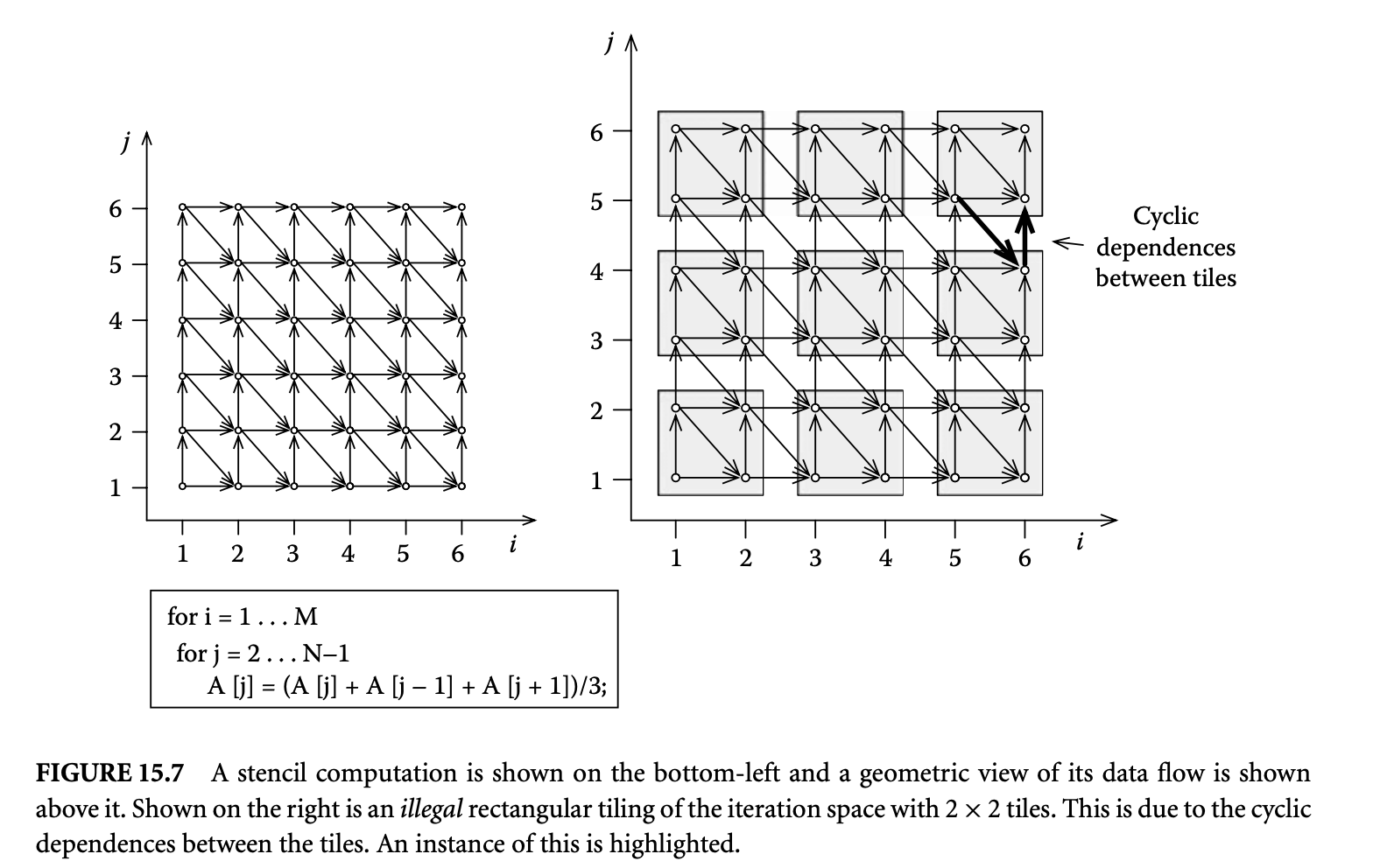 A dependence vector for an -dimensional perfect loop nest is an -vector , where the th component corresponds to the th loop (counted from outermost to innermost). A distance vector is a dependence vector , that is, every component is an integer. A dependence distance is the distance between the iteration that produces a value and the iteration that consumes a value. Distance vectors represent this information. The dependence distance vector for a value produced at iteration and consumed at a later iteration is . The stencil computation given in Figure 15.7 has three dependences. The values consumed at an iteration are produced at iterations , , and . The corresponding three dependence vectors are and .
Tiling is an iteration reordering transformation. Tiling reorders the iterations to be executed in a block-by-block or tile-by-tile fashion. Consider the tiled iteration space shown in Figure 15.7 and the following execution order. Both the tiles and the points within a tile are executed in the lexicographic order. The tiles are also executed in an atomic fashion, that is, all the iterations in a tile are executed before any iteration of another tile. It is very instructive to pause for a moment and ask whether this tiled execution order preserves all the dependences of the original computation. One can observe that the dependence is not preserved, and hence the tiling is illegal. There exists a nice geometric way of checking the legality of a tiling. A given tiling is illegal if there exist cyclic dependences between tiles. An instance of this cyclic dependence is highlighted in Figure 15.7.
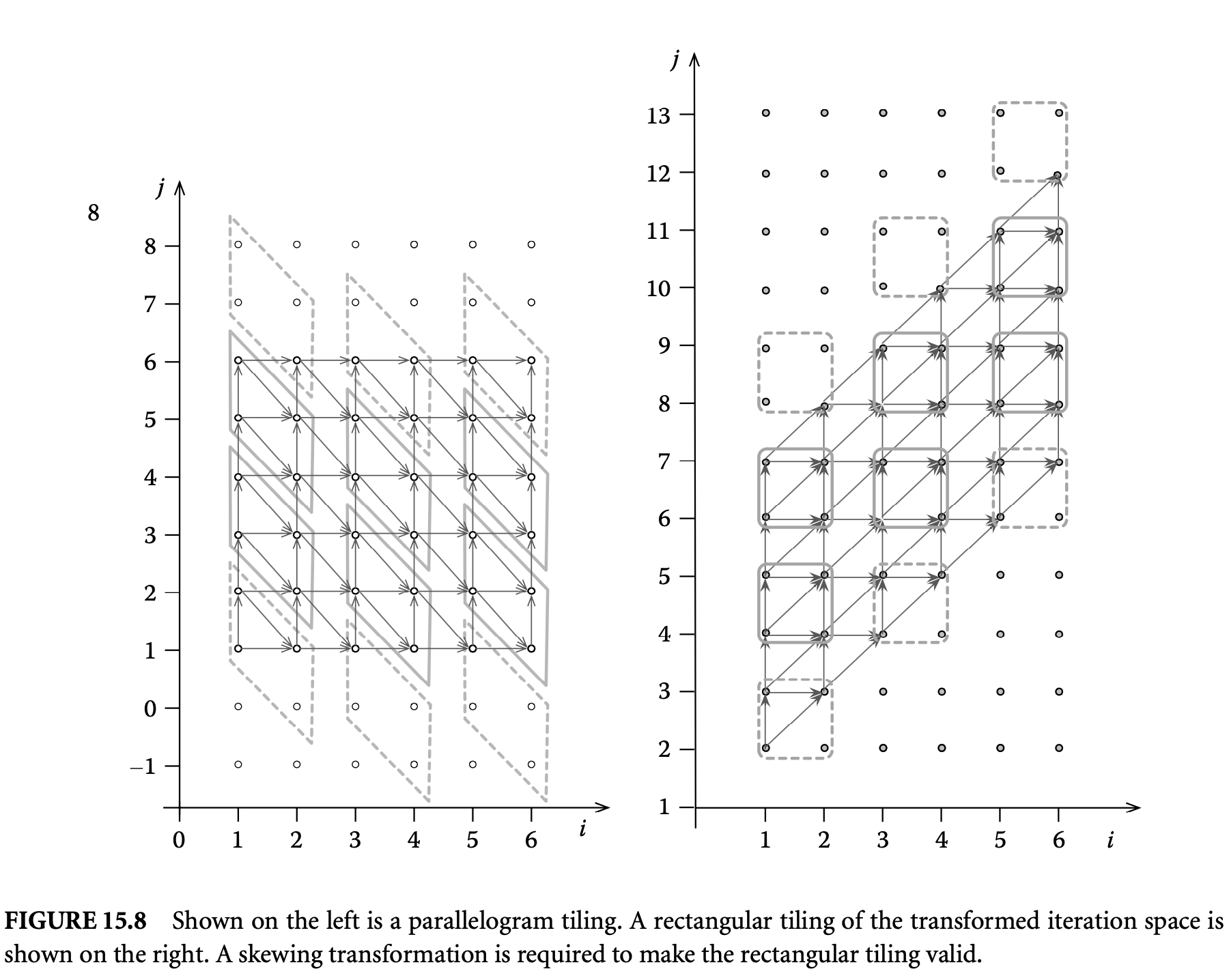
The legality of tiling is determined not by the dependences alone, but also by the shape of the tiles.10 We saw (Figure 15.7) that tiling the stencil computation with rectangles is illegal. However, one might wonder whether there are other tile shapes for which tiling is legal. Yes, tiling with parallelograms is legal as shown in Figure 15.8. Note how the change in the tile shape has avoided the cyclic dependences that were present in the rectangular tiling. Instead of considering nonrectangular shapes that make tiling legal, one could also consider transforming the data dependences so that rectangular tiling becomes legal. Often, one can easily find such transformations. A commonly used transformation is skewing. The skewed iteration space is shown in Figure 15.8 together with a rectangular tiling. Compare the dependences between tiles in this tiling with those in the illegal rectangular tiling shown in Figure 15.7. One could also think of more complicated tile shapes, such as hexagons or octagons. Because of complexity of tiled code generation such tile shapes are not used.
Legality of tiling also depends on the shape of the iteration space. However, for practical applications, we can check the legality with the shape of the tiles and dependence information alone.
A given tiling can be characterized by the shape and size of the tiles, both of which can be concisely specified with a matrix. Two matrices, clustering and tiling, are used to characterize a given tiling. The clustering matrix has a straightforward geometric interpretation, and the tiling matrix is its inverse and is useful in defining legality conditions. A parallelogram (or a rectangle) has four vertices and four edges. Let us pick one of the vertices to be the origin. Now we have two edges or two vertices adjoining the origin. The shape and size of the tiles can be specified by characterizing these edges or vertices. We can easily generalize these concepts to higher dimensions. In general, an -dimensional parallelepiped has vertices and facets (higher-dimensional edges), out of which facets and vertices adjoin the origin. A clustering matrix is an square matrix whose columns correspond to the facets that determine a tile. The clustering matrix has the property that the absolute value of its determinant is equal to the tile volume.
The clustering matrices of the parallelogram and rectangular tilings shown in Figure 15.8 are
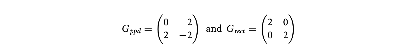
the first column represents the horizontal edge, and the second represents the oblique edge. In , the first column represents the horizontal edge, and the second represents the vertical edge.
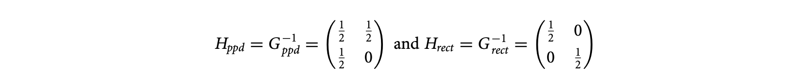
The tiling matrix is the inverse of the clustering matrix. The tiling matrices of the parallelogram and the rectangular tilings shown in Figure 15.8 are
 For rectangular tiling the edges are always along the canonical axes, and hence, there is no loss of generality in assuming that the tiling and clustering matrices are diagonal. The tiling is completely described by just the so-called tile size vector, , where each denotes the tile size along the th dimension. The clustering and tiling matrices are simply and , where denotes the diagonal matrix with as the diagonal entries.
A geometric way of checking the legality of a given tiling was discussed earlier. One can derive formal legality conditions based on the shape and size of the tiles and the dependences. Let be the set of dependence distance vectors. A vector is lexicographically nonnegative if the leading nonzero component of the is positive, that is, or both and . The floor operator when used on vectors is applied component-wise, that is, . The legality condition for a given (rectangular or parallelepiped) tiling specified by the tiling matrix and dependence set is
 The above condition formally captures the presence or absence of cycles between tiles.
We can now apply this legality condition to the stencil computation example. Let , the set of dependence vectors from the original or given stencil computation, and , the dependence vectors obtained after applying the skewing transformation to the original dependences. Earlier we showed that rectangular tiling of the original iteration space is not legal based on the existence of cycles between tiles (cf. Figure 15.7). This can also be verified by observing that the condition for validity, , is not satisfied, since, for the dependence vector in , we have . However, for the same dependences, , as shown in Figure 15.8, a parallelogram tiling is valid. This validity is confirmed by the satisfaction of the constraint . We also showed that a skewing transformation of the iteration space can make rectangular tiling valid. This can also be verified by observing the satisfaction of . In the case of rectangular tiling the legality condition can be simplified by using the fact that the tiling can be completely specified by the tile size vector . The legality condition for rectangular tiling specified by the tile size vector for a loop nest with a set of dependences is
 A rectangular tiling can also be viewed as a sequence of two transformations: strip mining and loop interchange. This view is presented by Raman and August in this text [84].
15.3.1.2 Optimal Tiling
Selecting the tile shape and selecting the sizes are two important tasks in using loop tiling. If rectangular tiling is valid or could be made valid by appropriate loop transformation, then it should be preferred over parallelepipeds. This preference is motivated by the simplicity and efficiency in tiled code generation as well as tile size selection methods. For many practical applications we can transform the loop so that rectangular tiling is valid. We discuss rectangular tiling only. Having fixed the shape of tiles to (hyper-)rectangles, we address the problem of choosing the "best" tile sizes.
Tile size selection methods vary widely depending on the purpose of tiling. For example, when tiling for multi-processor parallelism, analytical models are often used to pick the best tile sizes. However, when tiling for caches or registers, empirical search is often the best choice. Though the methods vary widely, they can be treated in the single unifying formulation of constrained optimization problems. This approach is used in the next section to formulate the optimal tile size selection problem.
Optimal Tile Size Selection ProblemThe optimal tile size selection problem involves selecting the best tile sizes from a set of valid tile sizes. What makes a tile size valid and what makes it the best can be specified in a number of ways. Constrained optimization provides this unified approach. Validity is specified with a set of constraints, and an objective function is used to pick the best tile sizes. A constrained optimization problem has the following form:

where is the variable, is the objective function, and are constraints on . The solution to such an optimization problem has two components: (a) the minimum value of over all valid and (b) a minimizer, which is a value of at which attains the minimum value.
All the optimal tile size selection problems can be formulated as a constrained optimization problem with appropriate choice of the and s. Furthermore, the structure of and s determines the techniques that can be used to solve the optimization problem. For example, consider the problem of tiling for data locality, where we seek to pick a tile size that minimizes the number of cache misses. This can be cast into an optimization problem, where the objective function is the number of misses, and the constraints are the positivity constraints on the tile sizes and possibly upper bounds on the tile sizes based on program size parameters as well as cache capacity. In the next two sections, we will present an optimization-based approach to optimal tile size selection in the context of two problems: (a) tiling for data locality and (b) tiling for parallelism. The optimization problems resulting from optimal tiling formulations can be cast into a particular form of numerical convex optimization problems called geometric programs, for which powerful and efficient tools are widely available. We first introduce this class of convex optimization problems in the next section and use them in the later sections.
15.3.1.2.2 Geometric Programs
In this section we introduce the class of numerical optimization problems called geometric programs, which will be used in later sections to formulate optimal tile size selection problems.
Let denote the vector of real, positive variables. A function is called a posynomial function of if it has the form
 where and . Note that the coefficients must be nonnegative, but the exponents can be arbitrary real numbers, including negative or fractional. When there is exactly one nonzero term in the sum, that is, and , we call a monomial function. For example, is a posynomial (but not monomial), is a monomial (and, hence, a posynomial), while is neither. Note that posynomials are closed under addition, multiplication, and nonnegative scaling. Monomials are closed under multiplication and division.
A geometric program (GP) is an optimization problem of the form
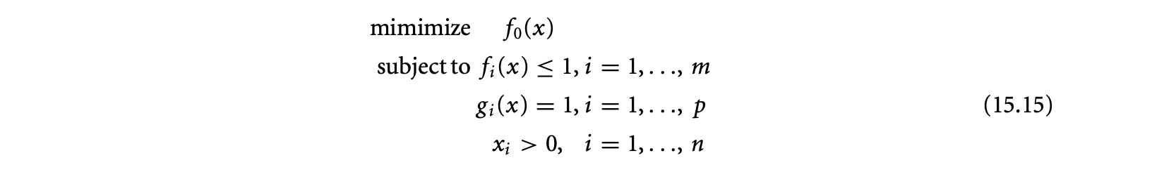
where are posynomial functions and are monomial functions. If, we call the GP an integer geometric program (IGP).
15.3.1.2.2.1 Solving IGPs
GPs can be transformed into convex optimization problems using a variable substitution and solved efficiently using polynomial time interior point methods. Integer solutions can be found by using a branch-and-bound algorithm. Tools such as YALMIP provide a high-level symbolic interface (in MATLAB) that can be used to define and solve IGPs. The number of (tile) variables of our IGPs are related to number of dimensions tiled and hence are often small. In our experience with solving IGPs related to tiling, the integer solutions were found in a few (fewer than 10) iterations of the branch-and-bound algorithm. The (wall clock) running time of this algorithm was just a few seconds, even with the overhead of using the symbolic MATLAB interface.
15.3.1.2.3 Tiling for Parallelism
We consider a distributed memory parallel machine as the execution target. Message passing is a widely used interprocess communication mechanism for such parallel machines. The cost of communication in such systems is significant. Programs with fine-grained parallelism require frequent communications and are not suited for message-passing-style parallel execution. We need to increase the granularity of parallel computation and make the communications less frequent. Tiling can be used to increase the granularity of parallelism from fine to coarse. Instead of executing individual iterations in parallel, we can execute tiles in parallel, and instead of communicating after every iteration, we communicate between tiles. The tile sizes determine how much computation is done between communications.
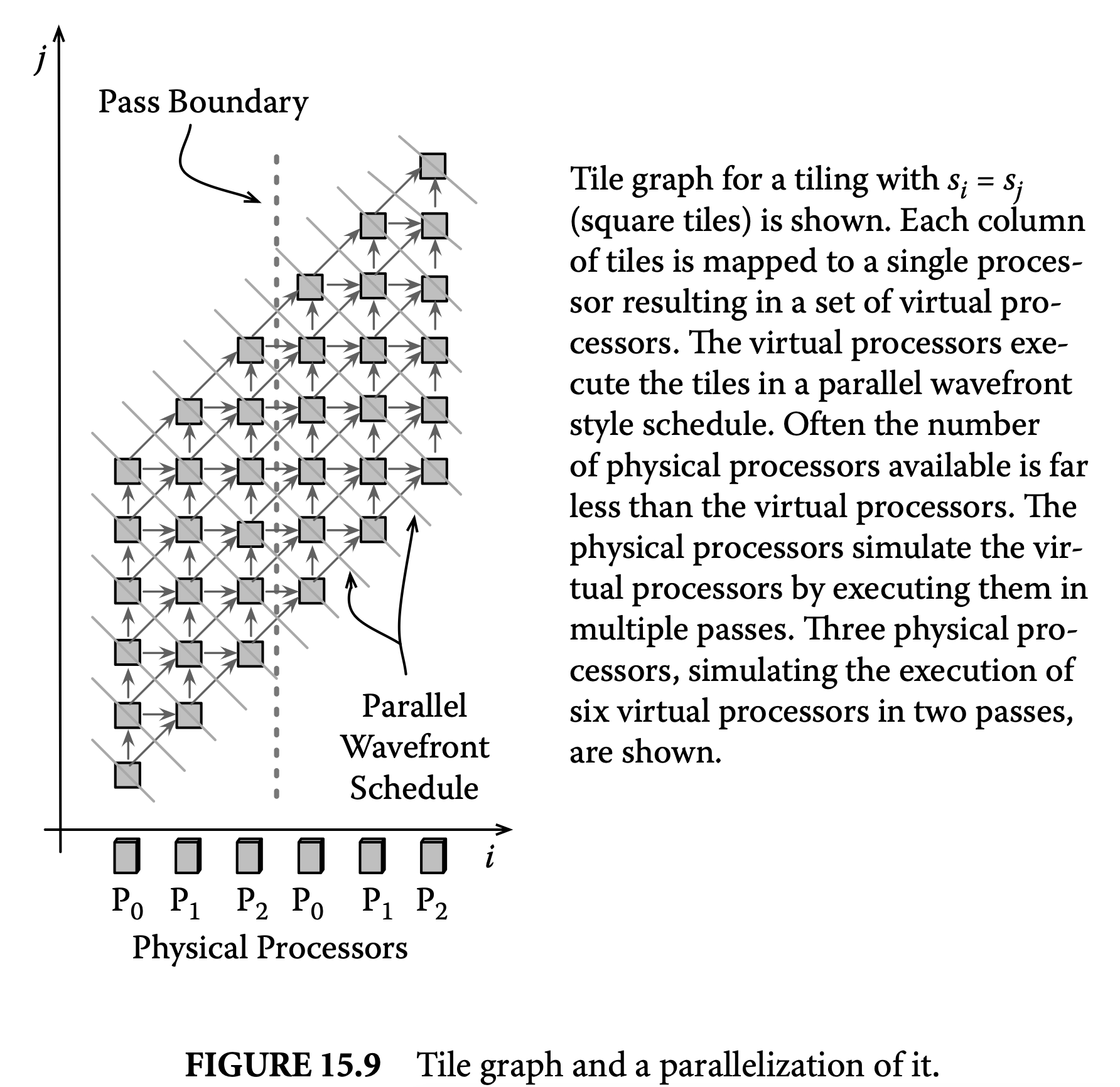
Consider the rectangular tiling shown in Figure 15.8. We seek to execute the tiles in parallel. To do this we need (a) a processor mapping that maps tiles to processors and (b) a schedule that specifies a (parallel) time stamp for each tile. A parallelization of a tiled iteration space involves derivation of a processor mapping and a schedule. A better abstraction of the tiled iteration space useful in comparing and analyzing different parallelizations is the tile graph. A tile graph consists of nodes that are tiles and edges representing dependences between them. Figure 15.9 shows the tile graph of the tiling shown in Figure 15.8. The dependences between tiles are induced by the dependences between the iterations and the tiles they are grouped into. The shape of the tile graph is determined by the shape of the tiled iteration space as well as the tile sizes. The shapes of the tile graph (Figure 15.9) and the rectangular tiled iteration space (Figure 15.8) are the same because the tile sizes are the same. It is useful to pause for a moment and think of the tile graph shape when and .
To parallelize the tile graph we need to find a parallel schedule and a processor mapping. As shown in Figure 15.9, the wavefronts corresponding to the lines define a parallel schedule -- all the tiles on a wavefront can be executed in parallel. We can verify that this schedule is valid by observing that any given tile is scheduled after all the tiles it depends on are executed. A processor mapping is valid if it does not map two tiles scheduled to execute at the same time to the same processor. There are many valid processor mappings possible for this schedule. For example, one can easily verify that the following three mappings are valid: (a) map each column of tiles to a processor, (b) map each row of tiles to a processor, and (c) map all the tiles along the diagonal line to a single processor. Though all of them are valid, they have very different properties: the first (column-wise) and the last (diagonal) map the same number of tiles to each processor, whereas the second (row-wise) maps a different number of tiles to different processors. For a load-balanced allocation one would prefer the column-wise or the diagonal mappings. However, for simplicity of the resulting parallel program, one would prefer the column-wise over the diagonal mapping.
Typically the number of processors that results from a processor mapping is far greater than the number of available processors. We call the former the virtual processors and the latter the physical processors. Fewer physical processors simulate the execution of the virtual processors in multiple passes. For example, the column-wise mapping in Figure 15.9 results in six virtual processors, and they are simulated by three physical processors in two passes. Tiles are executed in an atomic fashion; all the iterations in a tile are executed before any iteration of another tile. The parallel execution proceeds in a wavefront style.
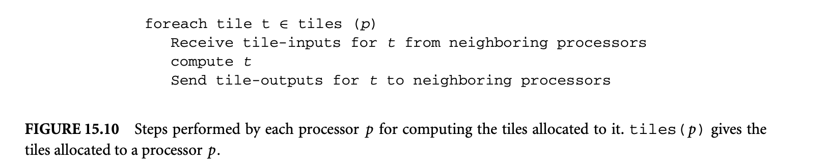 We call a parallelization idle-free if it has the property that once a processor starts execution it will never be idle until it finishes all the computations assigned to it. We call a parallelization load-balanced if it has the property that all the processors are assigned an (almost) equal amount of work. For example, the column-wise and diagonal mappings are load-balanced, whereas the row-wise mapping is not. Furthermore, within a given pass, the wavefront schedule is idle-free. Across multiple passes, it will be idle-free if by the time the first processor finishes its first column of tiles the last processor finishes at least one tile. This will be true whenever the number of tiles in a column is more than the number of physical processors.
15.3.1.2.4 An Execution Time Model
After selecting a schedule and a processor mapping, the next step is to pick the tile size. We want to pick the tile size that minimizes the execution time. We will develop an analytical model for the total running time of the parallel program and then use it to formulate a constrained optimization problem, whose solution will yield the optimal tile sizes.
We choose the wave front schedule and the column-wise processor mapping discussed earlier. Recall that the column-wise mapping is load-balanced, and within a pass the wave front schedule is idle-free. To ensure that the schedule is also idle-free across passes, we will characterize and enforce the constraint that the number of tiles in a column is greater than the number of physical processors. Furthermore, we consider the following receive-compute-send execution pattern (shown in Figure 10): every processor first receives all the inputs it needs to execute a tile and then executes the tiles and then sends the tile outputs to other processors. The total execution time is the time elapsed between the start of the first tile and the completion of the last tile. Let us assume that all the passes are full, that is, in each pass all the processors have a column of tiles to execute. Now, the last tile will be executed by the last processor, and its completion time will give the total execution time. Given that the parallelization is idle-free, the total time taken by any processor is equal to the initial latency (time it waits to get started) and the time it takes to compute all the tiles allocated to it. Hence, the sum of the latency and the computation time of the last processor is equal to the total execution time. Based on this reasoning, the total execution time is

where denotes the latency last processor to start, denotes the number of tiles allocated per processor, and is the time to execute a tile (sequentially) by a single processor. Here, the term denotes the time any processor takes to execute all the tiles allocated to it. Given that we have a load-balanced processor mapping, this term is same for all processors. In the following derivations, is the number of physical processors, and denote the size of the iteration space along and , respectively, and and are the tile sizes along and , respectively.
Let us now derive closed-form expressions for the terms discussed above. The time to execute a tile, , is the sum of the computation and communication time. The computation time is proportional to the area of the rectangular tile and is given by . The constant denotes the average time to execute one iteration. The communication time is modeled as an affine function of the message size. Every processor receives the left edge of the tile from its left neighbor and sends its right edge to the right neighbor. This results in two communications with messages of size , the length of the vertical edge of
a tile. The cost of sending a message of size is modeled by , where and are constants that denote the transmission cost per byte and the start-up cost of a communication call, respectively. The cost of the two communications performed for each tile is . The total time to execute a tile is now .
The number of tiles allocated to a processor is equal to the number of columns allocated to a processor times the number of tiles per column. The number of columns is equal to the number of passes, which is . The tiles per column is equal to , which makes .
The dependences in the tile graph induce the delay between the start of the processors. The slope , known as the rise, plays a fundamental role in determining the latency. The last processor can start as soon as the processor before it completes the execution of its first two tiles. Formally, the last processor can start its first tile only after . For example, in Figure 15.9 the last processor can start only after four time steps since and , yielding . Since at each time step a processor computes a tile, gives the time after which the last processor can start, that is, .
To ensure that there is no idle time between passes, we need to constrain the tile sizes such that by the time the first processor finishes its column of tiles, the last processor must have finished its first tile. The time the first processor takes to complete a column of tiles is equal to , and the time by which the last processor would finish its first tile is . The no idle time between passes constraint is .
Using the terms derived above we can now formulate an optimization problem to pick the optimal tile size.
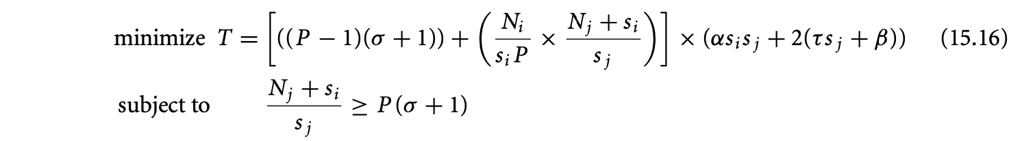 The solution to the above optimization problem yields the optimal tile sizes, that is, the tile sizes that minimize the total execution time of the parallel program, subject to the constraint that there is no idle time between passes.
The optimization problem in Equation 15.16 can be transformed into a GP. The objective function is directly a posynomial. With the approximation of , the constraint transforms into

which is the required form for a GP constraint. Adding to it the obvious constraints that tile sizes are integers and positive, that is, , and , we get an IGP that can be solved efficiently as discussed above. The solution to this IGP will yield the optimal tile sizes.
15.3.1.2.4.1 Generality of Approach
The analysis techniques presented above can be directly extended to higher-dimensional rectangular or parallelepiped iteration spaces. For example, stencil computations with two-dimensional or three-dimensional data grids, after skewing to make rectangular tiling valid, have parallelepiped iteration spaces, and the techniques described above can be directly applied to them. The GP-based modeling approach is quite general. Because of the fundamental positivity property of tile sizes, often the functions used in modeling parallel execution time or communication or computation volumes are posynomials. This naturally leads to optimization problems that are GPs.
15.3.1.2.5 Tiling for Data Locality
Consider the stencil computation shown in Figure 15.7. Every value, , computed at an iteration is used by three other computations as illustrated in the geometric view shown in Figure 15.7 (left).
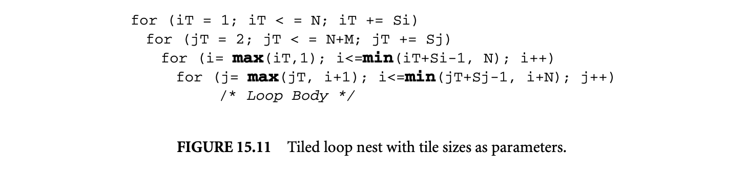 The three uses are in iterations and . Consider the case when the size of A is much larger than the cache size. On the first use at iteration , the value will be cache. However, for the other two uses, and , the value may not be in cache, resulting in a cache miss. This cache miss can be avoided if we can keep the computed values in the cache until their last use. One way to achieve this is by changing the order of the computations such that the iterations that use a value are computed "as soon as" the value itself is computed. Tiling is widely used to achieve such reorderings that improve data locality. Furthermore, the question of how soon the iterations that use a value should be computed is dependent on the size of the cache and processor architecture. This aspect can be captured by appropriately picking the tile sizes.
Consider the rectangular tiling of the skewed iteration space shown in Figure 15.8 (right). Figure 15.11 shows the tiled loop nest of the skewed iteration space, with tile sizes as parameters. The new execution order after tiling is as follows: both the tiles and the points within a tile are executed in column-major order. Observe how the new execution order brings the consumers of a value closer to the producer, thereby decreasing the chances of a cache miss. Figure 15.8 (right) shows a tiling with tiles of sizes . In general, the sizes are picked so that the volume data touched by a tile, known as its footprint, fits in the cache, and some metric such as number of misses or total execution time is minimized. A discussion of other loop transformations (e.g., loop fusion, fission, etc.) aimed at memory hierarchy optimization can be found in the chapter by Raman and August [84] in the same text.
15.3.1.2.5.1 Tile Size Selection Approaches
A straightforward approach for picking the best tile size is empirical search. The tiled loop nest is executed for a range of tile sizes, and the one that has the minimum execution time is selected. This search method has the advantage of being accurate, that is, the minimum execution time tile is the best for the machine on which it is obtained. However, such a search may not be feasible because of the huge space of tile sizes that needs to be explored. Often, some heuristic model is used to narrow down this space. In spite of the disadvantages, such an empirical search is the popular and widely used approach for picking the best tile sizes. For the obvious reason of huge search time, such an approach is not suitable for a compiler.
Compilers trade off accuracy for search time required to find the best tile size. They use approximate cache behavior models and high-level execution time models. Efficiency is achieved by specializing the tile size search algorithm to the chosen cache and execution time models. However, such specialization of search algorithms makes it difficult to change or refine the models.
Designing a good model for the cache behavior of loop programs is hard, but even harder is the task of designing a model that would keep up with the advancements in processor and cache architectures. Thus, cache models used by compilers are often outdated and inaccurate. In fact, the performance of a tiled loop nest generated by a state-of-the-art optimizing compiler could be a few factors poorer than the one hand-tuned with an empirical search for best tile sizes. This has led to the development of the so-called auto-tuners, which automatically generate loop kernels that are highly tuned to a given architecture. Tile sizes are an important parameter tuned by auto-tuners. They use a model-driven empirical search to pick the tile sizes. Essentially they do an empirical search for the best tile size over a space of tile sizes and use an approximate model to prune the search space.
15.3.1.2.5.2 Constrained Optimization Approach
Instead of discussing specialized algorithms, we present a GP-based framework that can be used to develop models, formulate optimal tile size selection problems, and obtain the best tile sizes by using the efficient numerical solvers. We illustrate the use of the GP framework by developing an execution time model for the tiled stencil computation and formulating a GP whose solution will yield the optimal tile sizes. Though we restrict our discussion to this illustration-based presentation, the GP framework is quite general and can be used with several other models. For example, the models used in the IBM production compiler or the one used by the auto-tuner ATLAS can be transformed into the GP framework.
The generality and wide applicability of the GP framework stems from a fundamental property of the models used for optimal tile size selection. The key property is based on the following: tile sizes are always positive and all these models use metrics and constraints that are functions of the tile sizes. These functions of tile size variables often turn out to be posynomials. Furthermore, the closure properties of posynomials provide the ability to compose models. We illustrate these in the following sections.
15.3.1.2.5.3 An Analytical Model
We will first derive closed-form characterizations of several basic components related to the execution of a tiled loop and then use them to develop an analytical model for the total execution time. We will use the following parameters in the modeling. Some of them are features of processor memory hierarchy and others are a combination of processor and loop body features:
- : The average cost (in cycles) of computing an iteration assuming that the accessed data values are in the lowest level of cache. This can be determined by executing the loop for a small number of iterations, such that the data arrays fit in the cache, and taking the average.
- : The cost (in cycles) for moving a word from main memory to the lowest level of cache. This can be determined by the miss penalties associated with caches, translation look aside buffers, and so on.
- : The average cost (in cycles) to compute and check loop bounds. This can be determined by executing the loops without any body and taking the average.
- and : The capacity and line size, in words, of the lowest level of cache. These two can be directly determined from the architecture manual.
15.3.1.2.5.4 Computation Cost
The number of iterations computed by a tile is given by the tile area . If the data values are present in the lowest level of cache, then the cost of computing the iterations of a tile, denoted by , is , where is the average cost to compute an iteration.
15.3.1.2.5.5 Loop Overhead Cost
Tiling (all the loops of) a loop nest of depth results in loops of which the outer loops enumerate the tiles and the inner loops enumerate points in a tile. We refer to the cost for computing and testing loop bounds as the loop overhead cost. In general, the loop overhead is significant for tiled loops and needs to be accounted for in modeling the execution time. The loop overhead cost of a given loop is proportional to the number of iterations it enumerates. In general, , the loops bounds check cost, is dependent on the complexity of the loop bounds of a given loop. However, for notational and modeling simplicity we will use the same for all the loops. Now the product of with the number iterations of a loop gives the loop overhead of that loop.
Consider the tiled loop nest of the skewed iteration space shown in Figure 15.11. The total number of iterations enumerated by the tile-loops (iT and jT loops) is . The loop overhead of the tile-loops is . With the small overapproximation of partial tiles by full tiles, the number of iterations enumerated by the point-loops (i and j loops), for any given iteration of the outer tile-loops,is . The loop overhead of the point-loops is . The total loop overhead of the tiled loop nest is denoted by .
15.3.1.2.5.6 Footprint of a Tile
The footprint of a tile is the number of distinct array elements touched by a tile. Let us denote the footprint of a tile of size s by F(s). Deriving closed-form descriptions of F(s) for loop nests with an arbitrary loop body is hard. However, for the case when the loop body consists of references to arrays and the dependences are distance vectors, we can derive closed-form descriptions of F(s). However, for the case when the loop body contains affine references, deriving closed-form expressions for F(s) is complicated. We illustrate the steps involved in deriving F(s) for dependence distance vectors with our stencil computation example.
Consider the tiled stencil computation. Let s= be the tile size vector, where represents the tile size along i and along j. Each (nonboundary, full) tile executes iterations updating the values of the one-dimensional array A. The number of distinct values of A touched by a tile is proportional to one of its edges, namely, . One might have to store some intermediate values during the tiled execution, and these require an additional array of size . Adding these two together, we get . Note that F(s) takes into account the reuse of values. Loops with good data locality (i.e., with at least one dimension of reuse) have the following property: the footprint is proportional to the (weighted) sum of the facets of the tile. Note that our stencil computation has this property, and hence F(s) is the sum of the facets (here just edges) and . To maximize the benefits of data locality, we should make sure that the footprint F(s) fits in the cache.
15.3.1.2.5.7 Load Store Cost of a Tile
Earlier during the calculation of the computation cost, we assumed that the values are available in the lowest level of the cache. Now we will model the cost of moving the values between main memory and the lowest level of cache. To derive this cost we need a model of the cache. We will assume a fully associative cache of capacity C words with cache lines of size L words. is the cost of getting a word from the main memory to the cache. Ignoring the reuse of cache lines across tiles, F(s) provides a good estimated number of values accessed by a tile during its execution. Let be the number of cache lines needed for F(s). We have , where L is the cache line size. Then the load store cost of a tile, denoted by , is
15.3.1.2.5.8 Total Execution Time of a Tiled Loop Nest
The total execution time of the tiled loop nest is the sum of the time it takes to execute the tiles and the loop overhead. The time to execute the tiles can be modeled as the product of time to execute a tile times the number of tiles. For our stencil computation the iteration space is a parallelogram, and calculating the number of rectangles that cover it is a hard problem. However, we can use the reasonable approximation of to model the number of tiles, denoted by ntiles (s). The total execution time T is given by
 where ntiles (s) is the number of tiles, is the cost of executing a tile, is the load store cost, and is the loop overhead.
15.3.1.2.5.9 Optimal Tile Size Selection Problem Formulation
Using the quantities derived above, we can now formulate an optimization problem whose solution will yield the optimal tile size - one that minimizes the total execution time. Recall that the function T (Equation 15.17) derived above models the execution time under the assumption that the data accessed by a tile fits in the cache. We model this assumption by translating it into a constraint in the optimization problem. Recall that F(s) measures the data accessed by a tile, and gives the number of cache lines needed for F(s). The constraint , where C is the cache capacity, ensures that all the data touched by a tile fits in the cache. Now we can formulate the optimization problem to find the tile size that minimizes as follows:
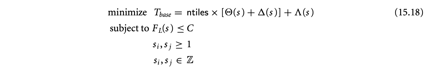 where the last two constraints ensure that and are positive and are integers.
15.3.1.2.5.10 Optimal Tiling Problem Is an IGP
The constrained optimization problem formulated above (Equation 15.18) can be directly cast into an IGP (integer geometric program) of the form of Equation 15.15. The constraints are already in the required form. The objective function is a posynomial. This can be easily verified by observing that the terms used in the construction of , namely, , and , are all posynomials, and posynomials are closed under addition -- the sum of posynomials is a posynomial. Based on the above reasoning, the optimization problem Equation 15.18 is an IGP.
15.3.1.2.5.11 A Sophisticated Execution Time Model
One can also consider a sophisticated execution time model that captures several hardware and compiler optimizations. For example, modern processor architectures support nonblocking caches, out-of-order issue, hardware prefetching, and so on, and compilers can also do latency hiding optimizations such as software prefetching and instruction reordering. As a result of these hardware and compiler optimizations, one can almost completely hide the load-store cost. In such a case, the cost of a tile is not the sum of the computation and communication cost, but the maximum of them. We model this sophisticated execution time with the function as follows:

Thanks to our unified view of the optimization problem approach, we can substitute with in the optimization problem Equation 15.18 and solve for the optimal tile sizes. However, must be a posynomial for this substitution to yield a GP. We can easily transform to a posynomial by introducing new variables to eliminate the operator.
15.3.1.3 Tiled Code Generation
An important step in applying the tiling transformation is the generation of the tiled code. This step involves generation of tiled loops and the transformed loop body. Since tiling can be used for a variety of purposes, depending on the purpose, the loop body generation can be simple and straightforward to complicated. For example, loop body generation is simple when tiling is used to improve data cache locality, whereas, in the context of register tiling, loop body generation involves loop unrolling followed by scalar replacement, and in the context of tiling for parallelism, loop body generation involves generation of communication and synchronization. There exist a variety of techniques for loop body generation, and a discussion of them is beyond the scope of this article. We will present techniques that can be used for tiled loop generation both when the tile sizes are fixed and when they are left as symbolic parameters.
15.3.1.3 Tiled Loop Generation
We will first introduce the structure of tiled loops and develop an intuition for the concepts involved in generating them. Consider the iteration space of a two-dimensional parallelogram such as the one shown in Figure 15.12, which is the skewed version of the stencil computation. Figure 15.13 shows a geometric view of the iteration space superimposed with a rectangular tiling. There are three types of tiles: full (which are completely contained in the iteration space), partial (which are not completely contained but have a nonempty intersection with the iteration space), and empty (which do not intersect the iteration space).
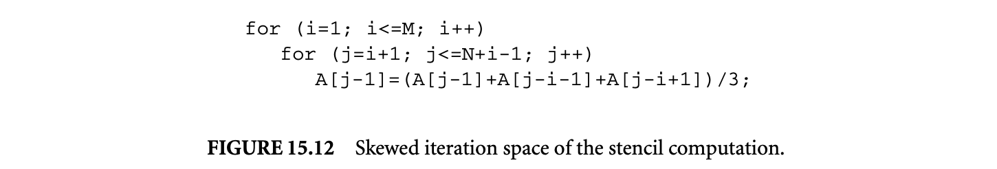 The lexicographically earliest point in a tile is called its origin. The goal is to generate a set of loops that scans (i.e., visits) each integer point in the original iteration space based on the tiling transformation, where the tiles are visited lexicographically and then the points within each tile are visited lexicographically. We can view the four loops that scan the tiled iteration space as two sets of two loops each, where the first set of two loops enumerate the tile origins and the next set of two loops visit every point within a tile. We call the loops that enumerate the tile origins the tile-loops and those that enumerate the points within a tile the point-loops.
15.3.1.3.2 Bounding Box Method
One solution for generating the tile-loops is to have them enumerate every tile origin in the bounding box of the iteration space and push the responsibility of checking whether a tile contains a valid iteration to the point-loops. The tiled loop nest generated with this bounding box scheme is shown in Figure 15.11. The first two loops (iT and jT) enumerate all the tile origins in the bounding box of size , and the two inner loops (i and j) scan the points within a tile. A closer look at the point-loop bounds reveals its simple structure. One set of bounds is from what we refer to as the tile box bounds, which restrict the loop variable to points within a tile. The other set of bounds restricts the loop variable to points within
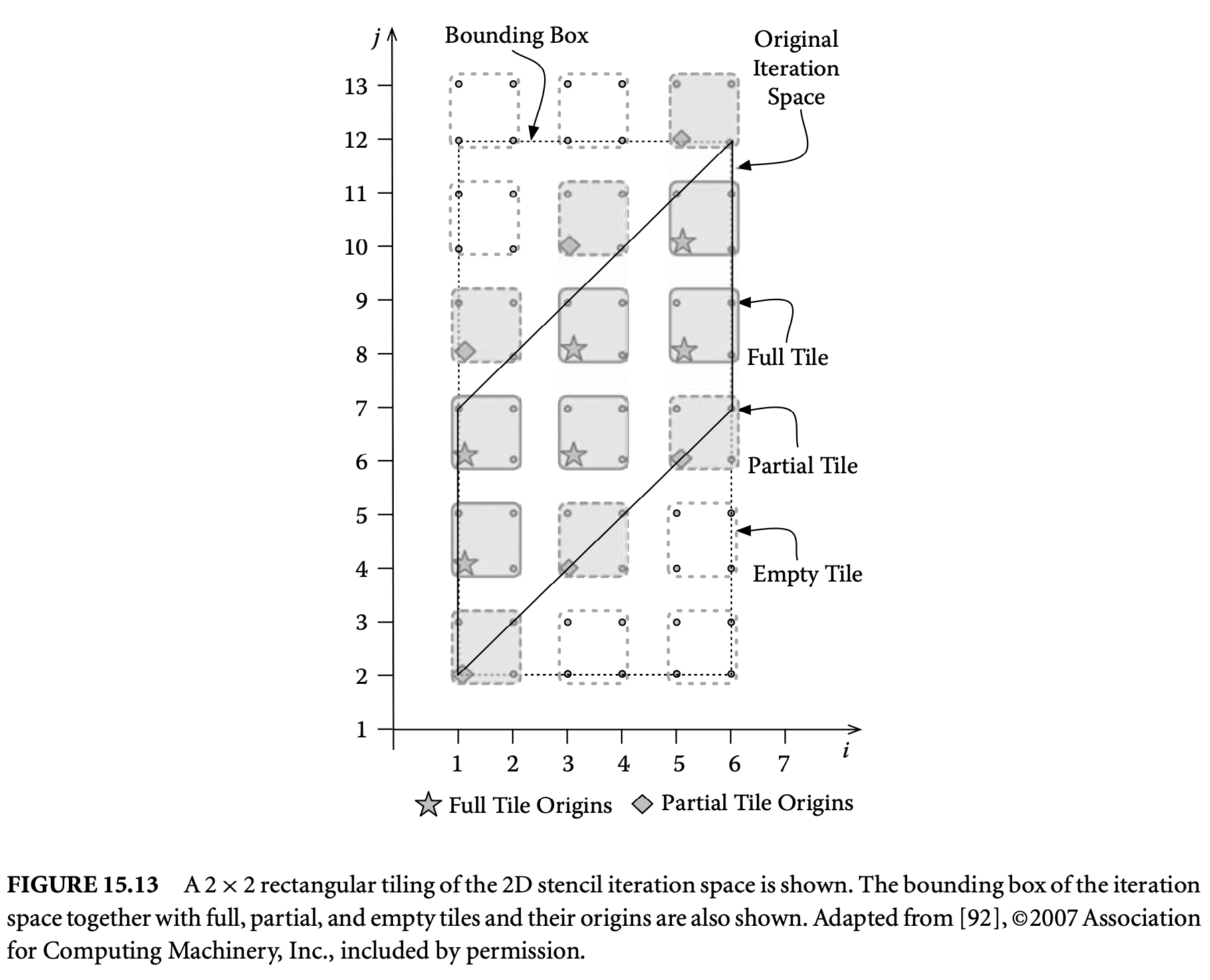
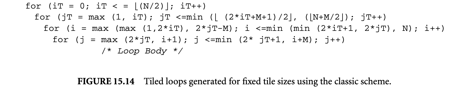
the iteration space. Combining these two sets of bounds, we get the point-loops that scan points within the iteration space and tiles. Geometrically, the point-loop bounds correspond to the intersection of the tile box (or rectangle) and the iteration space, here the parallelogram in Figure 15.13.
The bounding box scheme provides a couple of important insights into the tiled-loop generation problem. First, the problem can be decomposed into the generation of tile-loops and the generation of point-loops. Such a decomposition leads to efficient loop generation, since the time and space complexity of loop generation techniques is a doubly exponential function of the number of bounds. The second insight is the scheme of combining the tile box bounds and iteration space bounds to generate point-loops. An important feature of the bounding box scheme is that tile sizes need not be fixed at loop generation time, but can be left as symbolic parameters. This feature enables generation of parameterized tiled loops, which is useful in iterative compilation, auto-tuners, and runtime tile size adaptation. However, the empty tiles enumerated by tile-loops can become a source of inefficiency, particularly for small tile sizes.
15.3.1.3.3 When Tile Sizes Are Fixed
When the tile sizes can be fixed at the loop generation time, an exact tiled loop nest can be generated. The tile-loops are exact in the sense that they do not enumerate any empty tile origins. When the tile sizes are fixed, the tiled iteration space can be described as a set of linear constraints. Tools such as OMEGA and CLOOG provide standard techniques to generate loops that scan the integer points in sets described by linear constraints. These tools can be used to generate the tiled loop nest. The exact tiled loop nest for the two-dimensional stencil example is shown in Figure 15.14. Note that the efficiency due to the exactness of the tile-loops has come at the cost of fixing the tile sizes at generation time. Such loops are called fixed tiled loops.
The classic schemes for tiled loop generation take as input all the constraints that describe the bounds of the loops of the tiled iteration space, where is the depth of the original loop nest. Since the time-space complexity of the method is doubly exponential on the number of constraints, an increase in the number (from to ) of constraints might lead to situations where the loop generation time becomes prohibitively expensive. Similar to the bounding box technique, tiled loop generation for fixed tile sizes can also be decomposed into generating tile-loops and point-loops separately. Such a decomposition will reduce the number of constraints considered into each step by half and will improve the scalability of the tiled loop generation method.
15.3.2 Tiling Irregular Applications
Applications that make heavy use of sparse data structures are difficult to parallelize and reschedule for improved data locality. Examples of such applications include mesh-quality optimization, nonlinear equation solvers, linear equation solvers, finite element analysis, N-body problems, and molecular dynamics simulations. Sparse data structures introduce irregular memory references in the form of indirect array accesses (e.g., A[B[i]]), which inhibit compile-time, performance-improving transformations such as tiling. For example, in Figure 15.15, the array A is referenced with two different indirect array accesses, p[i] and q[i].
The flow, memory-based data dependences within the loop in Figure 15.15 can be described with the dependence relation (), where iteration depends on the value generated in iteration .


The uninterpreted functions and are static place holders for quantities that are unknown until runtime. It is not possible to parallelize or tile the loop in Figure 15.15 without moving some of the required analysis to the runtime.
To address this problem, inspector and executor strategies have been developed where the inspector dynamically analyzes memory reference patterns and reorganizes computation and data, and the executor executes the irregular computation in a different order to improve data locality or exploit parallelism. The ideal role for the compiler in applying inspector and executor strategies is performing program analysis to determine where such techniques are applicable and inserting inspector code and transforming the original code to form the executor. This section summarizes how inspector and executor strategies are currently applied to various loop patterns. The section culminates with the description of a technique called full sparse tiling being applied to irregular Gauss-Seidel.
15.3.2.1 Terminology
Irregular memory references are those that cannot be described with a closed-form, static function. Irregular array references often occur as a result of indirect array references where an access to an index array is used to reference a data array (e.g., A[p[i]] and A[q[i]] in Figure 15.15). A data array is an array that holds data for the computation. An index array is an array of integers, where the integers indicate indices into a data array or another index array.
This section assumes that data dependence analysis has been performed on the loops under consideration. The dependences are represented as relations between integer tuples with contraints specified using Presburger arithmetic including uninterpreted function symbols. Presburger arithmetic includes the universal operator , existential operator , conjunction , disjunction , negation , integer addition , and multiplication by a constant.
The dependence relations are divided into flow dependences, anti dependences, and output dependences. Flow dependence relations are specified as a set of iteration pairs where the iteration in which a read occurs depends on the iteration where a write occurs. The flow dependence relation for Figure 15.15 is as follows:

An anti dependence is when a write must happen after a read because of variable reuse. The anti dependence relation for the example in Figure 15.15 is
 An output dependence is a dependence between two writes to the same memory location. The output dependence relation for the example in Figure 15.15 is

A reduction loop has no loop-carried dependences except for statements of the form
 where X is a reference to a scalar or an array that is the same on the left- and right-hand side of the assignment, there are no references to the variable being referenced by X in the expression on the right-hand side, and op is an associative operator (e.g., addition, max, min). Since associative statements
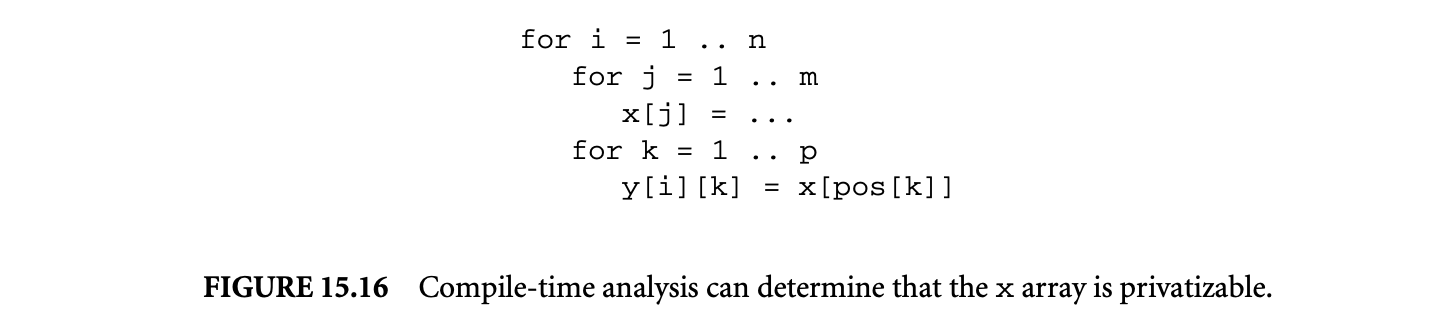 may be executed in any order, the loop may be parallelized as long as accesses to X are surrounded with a lock.
15.3.2.2 Detecting Parallelism
In some situations, static analysis algorithms are capable of detecting when array privatization and loop parallelization are possible in loops involving indirect array accesses. Figure 15.16 shows an example where compile-time program analysis can determine that the array x can be privatized, and therefore the i loop can be parallelized. The approach is to analyze the possible range of values that pos[k] might have and verify that it is a subset of the range [l..m], which is the portion of x being defined in the j loop.
If compile-time parallelism detection is not possible, then it is sometimes possible to detect parallelism at runtime. Figures 15.17 and 15.19 show loops where runtime tests might prove that the loop is in fact parallelizable. For the example in Figure 15.17, there are possible sets of flow and anti dependences between the write to A[p[i]] and the read of A[i]. If a runtime inspector determines that for all , is greater than , then the loop is parallelizable. Figure 15.18 shows an inspector that implements the runtime check and an executor that selects between the original loop and a parallel version of the loop.
To show an overall performance improvement, the overhead of the runtime inspector must be amortized over multiple executions of the loop. Therefore, one underlying assumption is that an outer loop encloses the loop to be parallelized. Another assumption needed for correctness is that the indirection arrays p and q are not modified within the loops. Figure 15.19 has an example where the inspection required might be overly cumbersome. In Figure 15.19, there are possible sets of flow and anti dependences between the write to A[p[i]] and the read of A[q[i]]. If it can be shown that for all and such that , is not equal to , then there are no dependences in the loop. Notice in Figure 15.20 that for this example, the inspector that determines whether there is a dependence requires time, thus making it quite difficult to amortize such parallelization detection for this example.
15.3.2.3 Runtime Reordering for Data Locality and Parallelism
Many runtime data reordering and iteration reordering heuristics for loops with no dependences or only reduction dependences have been developed. Such runtime reordering transformations inspect data mappings (the mapping of iterations to data) to determine the best data and iteration reordering within a parallelizable loop.
In molecular dynamics simulations there is typically a list of interactions between molecules, and each interaction is visited to modify the position, velocity, and acceleration of each molecule. Figure 15.21 outlines the main loop within the molecular dynamics benchmark moldyn. An outer time-stepping loop makes amortization of inspector overhead possible. The j loop calculates the forces on the molecules using the left and right index arrays, which indicate interaction pairs. In the j loop are two reduction
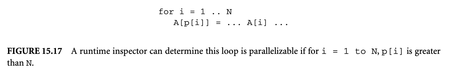
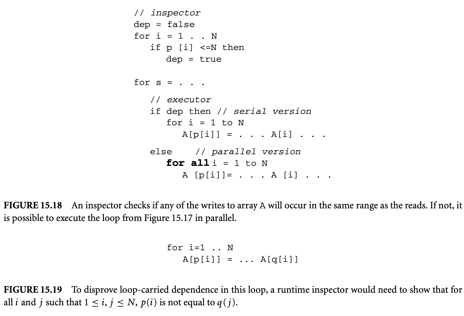
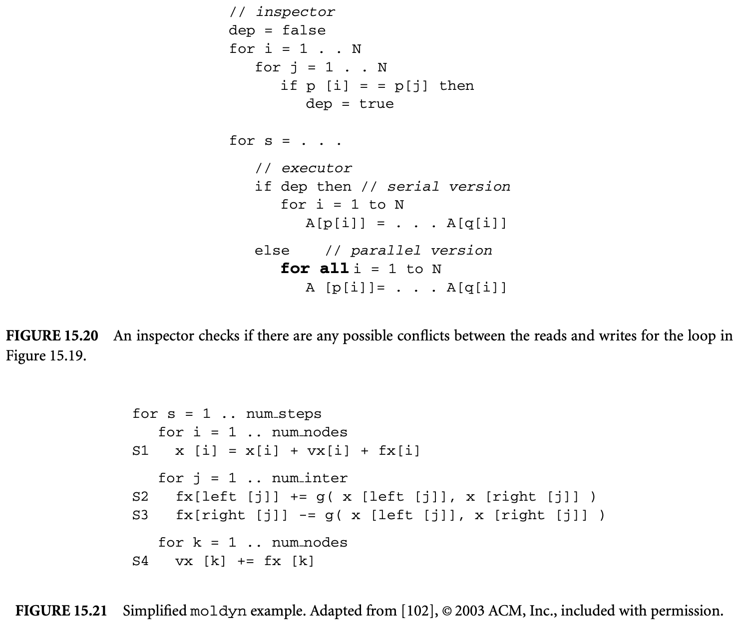
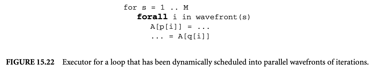
statements where the x-coordinate of the force fx for a molecule is updated as a function of the original x position for that molecule and the x position of some neighboring molecule right[i]. The j loop indirectly accesses the data arrays x and fx with the index arrays left and right.
Runtime data and iteration reorderings are legal for the j loop, because it only involves loop-carried dependences due to reductions. The data and iteration reordering inspectors can be inserted before the s loop, because the index arrays left and right are not modified within s (in some implementations of moldyn the index arrays are modified every 10 to 20 iterations, at which point the reorderings would need to be updated as well). The inspector can use various heuristics to inspect the index arrays and reorder the data arrays x and fx including: packing data items in the order they will be accessed in the loop, ordering data items based on graph partitioning, and sorting iterations based on the indices of the data items accessed. As part of the data reordering, the index arrays should be updated using a technique called pointer update. Iteration reordering is implemented through a reordering of the entries in the index array. Of course in this example, the left and right arrays must be reordered identically since entries left[i] and right[i] indicate an interacting pair of molecules. The executor is the original computation, which uses the reordered data and index arrays.
A significant amount of work has been done to parallelize irregular reduction loops on distributed memory machines. The data and computations are distributed among the processors in some fashion. Often the data is distributed using graph partitioning, where the graph arises from a physical mesh or list of interactions between entities. A common way to distribute the computations is called "owner computes," where all updates to a data element are performed by the processor where the data is allocated. Inspector and executor strategies were originally developed to determine a communication schedule for each processor so that data that is read in the loop is gathered before executing the loop, and at the end of the loop results that other processors will need in the next iteration are scattered. In iterative computations, an owner-computes approach typically involves communication between processors with neighboring data at each outermost iteration of the computation. The inspector must be inserted into the code after the index arrays have been initialized, but preferably outside of a loop enclosing the target loop. The executor is the original loop with gather and scatter sections inserted before and after.
For irregular loops with loop-carried dependences, an inspector must determine the dependences at runtime before rescheduling the loop. The goal is to dynamically schedule iterations into wavefronts such that all of the iterations within one wavefront may be executed in parallel. As an example, consider the loop in Figure 15.15. The flow, anti, and output dependences for the loop are given in Section 15.3.2.1. An inspector for detecting partial parallelism inspects all the dependences for a loop and places iterations into wavefronts. The original loop is transformed into an executor similar to the one in Figure 15.22, where the newly inserted s loop iterates over wavefronts, and all iterations within a wavefront can be executed in parallel.
15.3.2.4 Tiling Irregular Loops with Dependences11
Parts of this section are adapted from [102], ©ACM, Inc., included with permission, and from [101], with kind permission of Springer Science and Business Media © 2002.
The partial parallelism techniques described in Section 15.3.2.3 dynamically discover fine-grained parallelism within a loop. Sparse tiling techniques can dynamically schedule between loops or across outermost loops and can create course-grain parallel schedules. Two application domains where sparse tiling techniques have been found useful are iterative computations over interaction lists (e.g., molecular dynamics simulations) and iterative computations over sparse matrices. This section describes full sparse tiling, which
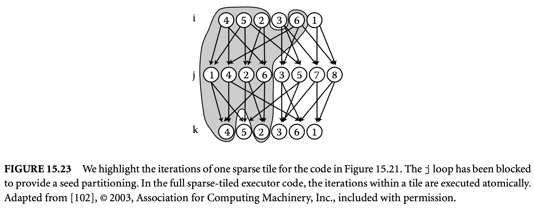 has been used to tile sparse computations across loops in a molecular dynamics benchmark and across the outermost loop of iterative computations.
15.3.2.4.1 Full Sparse Tiling for Molecular Dynamics Simulations
The runtime data and iteration reordering transformations described in Section 15.3.2 may be applied to the loop in the molecular dynamics code shown in Figure 15.21. Reordering the data and iterations within the loop is legal since the loop is a reduction. Full sparse tiling is capable of scheduling subsets of iterations across the , , and loops in the same example. The full sparse tiling inspector starts with a seed partitioning of iterations in one of the loops (or in one iteration of an outer loop). If other data and iteration reordering transformations have been applied to the loop being partitioned, then consecutive iterations in the loop have good locality, and a simple block partitioning of the iterations is sufficient to obtain an effective seed partitioning. Tiles are grown from the seed partitioning to the other loops involved in the sparse tiling by a traversal of the data dependences between loops (or between iterations of an outer loop). Growing from the seed partition to an earlier loop entails including in the tile all iterations in the previous loop that are sources for data dependences ending in the current seed partition and that have not yet been placed in a tile. Growth to a later loop is limited to iterations in the later loop whose dependences have been satisfied by the current seed partition and any previously scheduled tiles.
For the simplified example, Figure 15.23 shows one possible instance of the data dependences between iterations of the , , and loops after applying various data and iteration reorderings to each of the loops. A full sparse tiling iteration reordering causes subsets of all three loops to be executed atomically as sparse tiles. Figure 15.23 highlights one such sparse tile where the loop has been blocked to create a seed partitioning. The highlighted iterations that make up the first tile execute in the following order: iterations 4, 5, 2, and 6 in loop ; iterations 1, 4, 2, and 6 in loop ; and iterations 4 and 2 in loop . The second tile executes the remaining iterations. Figure 15.24 shows the executor that maintains the outer loop over time steps, iterates over tiles, and then within the , , and loops executes the iterations belonging
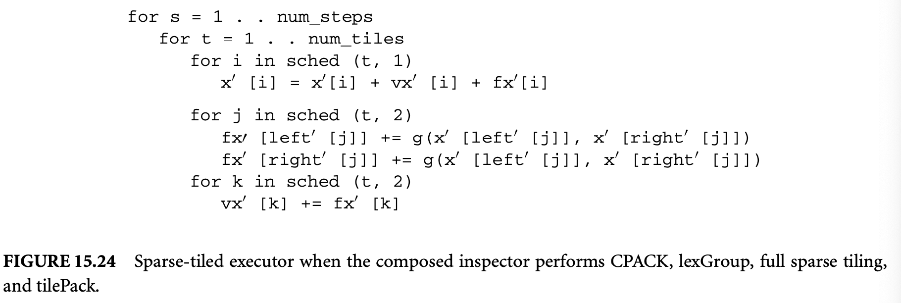
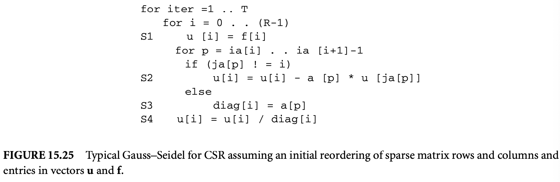
to each tile as specified by the schedule data structure. Since iterations within all three loops touch the same or adjacent data locations, locality between the loops is improved in the new schedule.
Full sparse tiling can dynamically parallelize irregular loops by executing the directed, acyclic dependence graph between the sparse tiles in parallel using a master-worker strategy. The small example shown in Figure 15.23 only contains two tiles, where one tile must be executed before the other to satisfy dependences between the , , and loops. In a typical computation where the seed partitions are ordered via a graph coloring, more parallelism between tiles is possible.
15.3.2.4.2 Full Sparse Tiling for Iterative Computations Over Sparse Matrices
Full Sparse tiling can also be used to improve the temporal locality and parallelize the Gauss-Seidel computation. Gauss-Seidel is an iterative computation commonly used alone or as a smoother within multigrid methods for solving systems of linear equations of the form , where is a matrix, is a vector of unknowns, and is a known right-hand side. Figure 15.25 contains a linear Gauss-Seidel computation written for the compressed sparse row (CSR) sparse matrix format. We refer to iterations of the outer loop as convergence iterations. The iteration space graph in Figure 15.26 visually represents an instance of the linear Gauss-Seidel computation. Each iteration point in the iteration space represents all the computation for the unknown at convergence iteration (one instance of S1 and S4 and multiple instances of S2 and S3). The iter axis shows three convergence iterations. The dark arrows show the data dependences between iteration points for one unknown in the three convergence iterations. The unknowns are indexed by a single variable , but the computations are displayed in a two-dimensional plane parallel to the and axes to exhibit the relationships between iterations. At each convergence iteration the relationships between the unknowns are shown by the lightly shaded matrix graph. Specifically, for each nonzero in the sparse matrix , , there is an edge in the matrix graph. The original
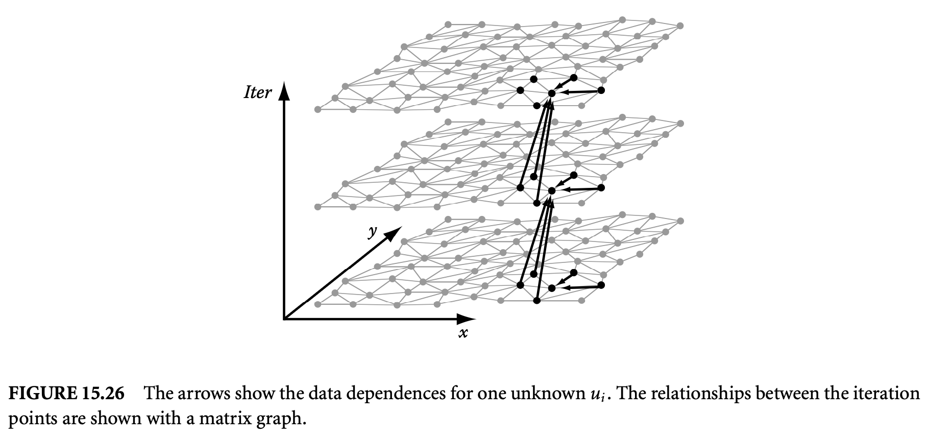
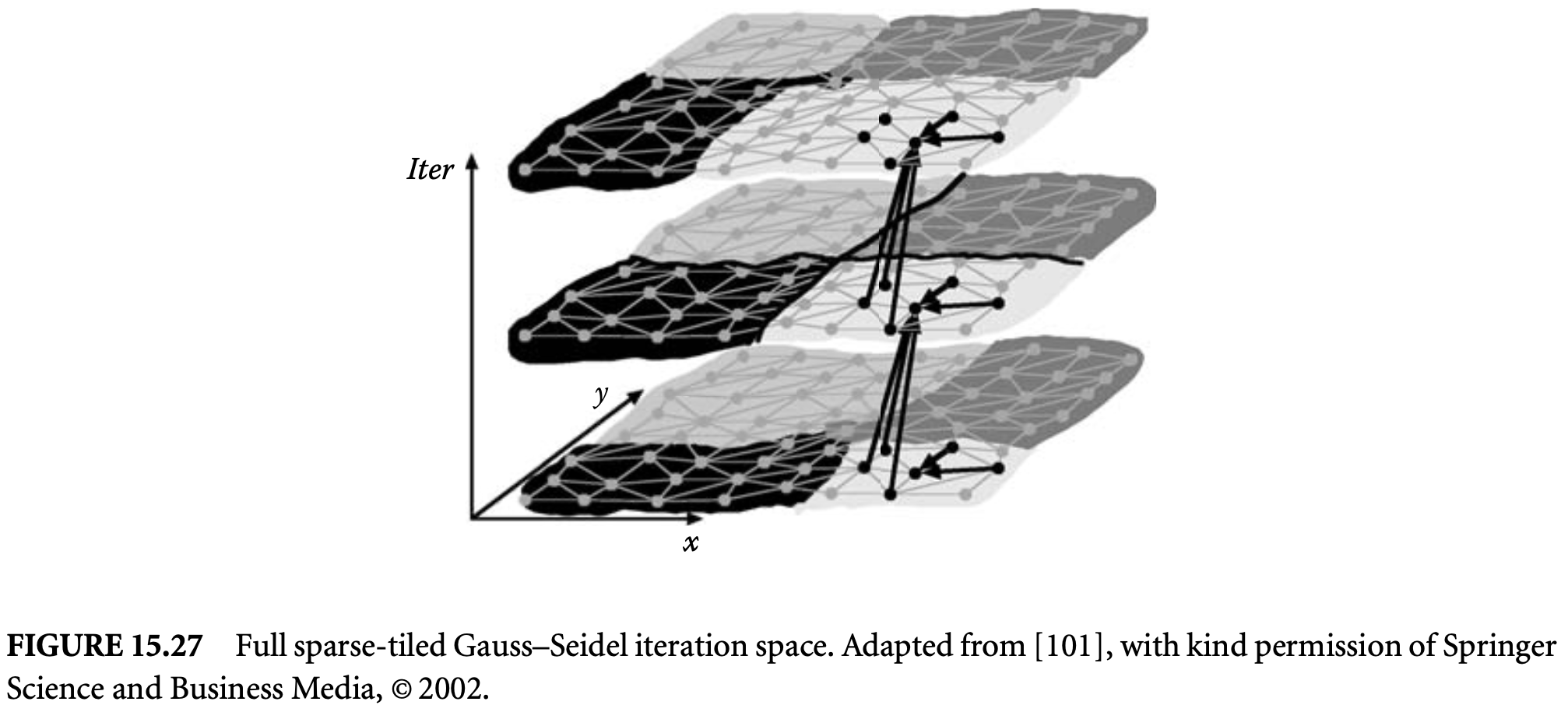
order, , given to the unknowns and corresponding matrix rows and columns is often arbitrary and can be changed without affecting the convergence properties of Gauss-Seidel. Therefore, if the unknowns are mapped to another order before performing Gauss-Seidel, the final numerical result will vary somewhat, but the convergence properties still hold.
In linear Gauss-Seidel, the data dependences arise from the nonzero structure of the sparse matrix . Each iteration point depends on the iteration points of its neighbors in the matrix graph from either the current or the previous convergence iteration, depending on whether the neighbor's index is ordered before or after . The dependences between iteration points within the same convergence iteration make parallelization of Gauss-Seidel especially difficult. Approaches to parallelizing Gauss-Seidel that maintain the same pattern of Gauss-Seidel data dependences use the fact that it is possible to apply an a priori reordering to the unknowns and the corresponding rows of the sparse matrix . This domain-specific knowledge is impossible to analyze with a compiler, so while automating full sparse tiling, it is necessary to provide some mechanism for a domain expert to communicate such information to the program analysis tool.
Figure 15.27 illustrates how the full sparse tiling inspector divides the Gauss-Seidel iteration space into tiles. The process starts by performing a seed partitioning on the matrix graph. In Figure 15.27, the seed-partitioned matrix graph logically sits at the second convergence iteration, and tiles are grown to the first and third convergence iterations.14 The tile growth must satisfy the dependences. For Gauss-Seidel, that involves creating and maintaining a new data order during tile growth. The full sparse tiling executor is a transformed version of the original Gauss-Seidel computation that executes each tile atomically (see Figure 15.28).
Footnote 14: The number of iterations for tile growth is usually small (i.e., two to five), and the full sparse tiling pattern can be repeated multiple times if necessary. The tile growth is started from a middle iteration to keep the size of the tiles as small as possible.
At runtime, the full sparse tiling inspector generates a data reordering function for reordering the rows and columns in the matrix, , and a tiling function, x . The tiling function maps iteration points to tiles. From this tiling function, the inspector creates a schedule function, x . The schedule function specifies for each tile and convergence iteration the subset of the reordered unknowns that must be updated. The transformed code shown in Figure 15.28 performs a tile-by-tile execution of the iteration points using the schedule function, which is created by the inspector to satisfy the following:

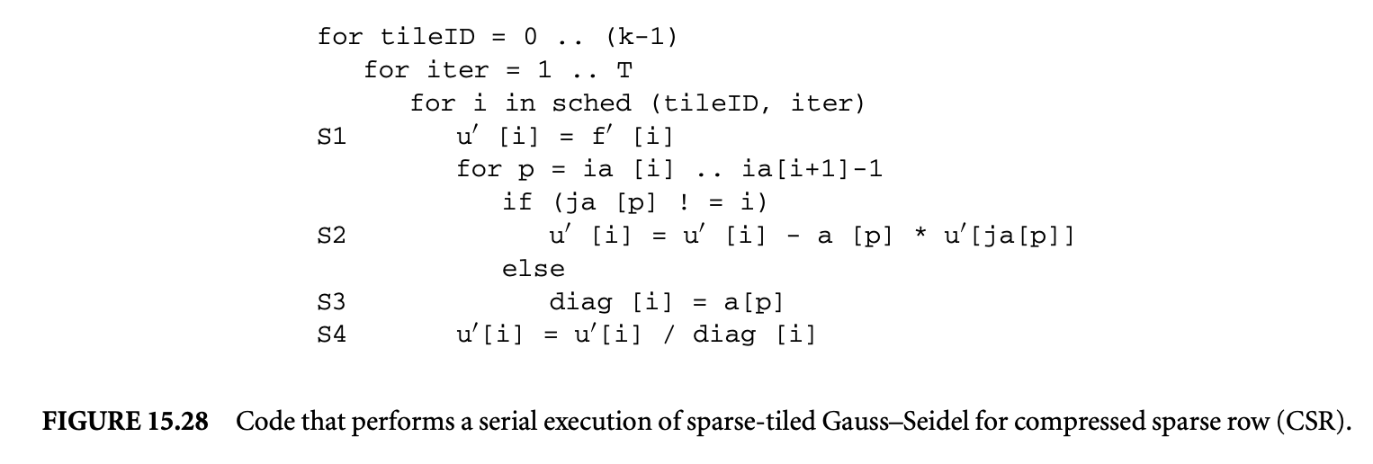
A matrix graph partitioning serves as a seed partitioning from which tiles can be grown. The seed partitioning determines the tiling at a particular convergence iteration, . Specifically at , where , the tiling function is set to the partition function, . To determine the tiling at other convergence iterations, the tile growth algorithm adds or deletes nodes from the seed partition as needed to ensure that atomic execution of each tile does not violate any data dependences.
The FullSparseNaive_GSCSR algorithm, shown in Figure 15.29, generates the tiling function for the Gauss-Seidel computation in Figure 15.25. While generating the tiling function, ordering constraints between nodes in the matrix graph are maintained in the relation NodeOrd. The first two statements in
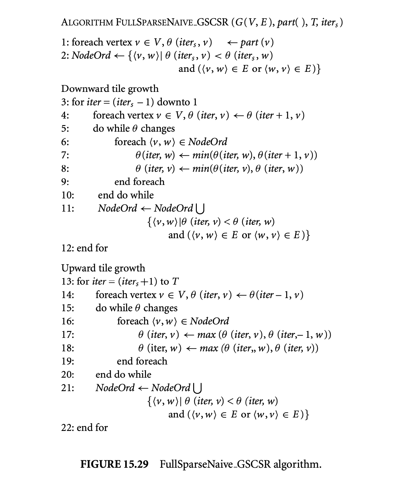 the algorithm initialize the NodeOrd relation and all of the tiling function values for the convergence iteration . The algorithm then loops through the convergence iterations such that , setting at each iteration point to . Finally, it visits the edges that have endpoints in two different partition cells, adjusting the tiling function to ensure that the data dependences are satisfied. The process is repeated for the convergence iterations between and in the upward tile growth. Once neighboring nodes, , are put into two different tiles at any iteration , the relative order between these two nodes must be maintained. The NodeOrd relation maintains that relative order. For example, if , then .
The running time of this algorithm is , where is the number of convergence iterations, is the number of tiles, is the number of nodes in the matrix graph, and is the number of edges in the matrix graph. The term is due to the while loops that begin at lines 5 and 15. In the worst case, the while loop will execute times, with only one value decreasing (or increasing in the forward tile growth) each time through the while loop. Each can take on values between 1 and , where is the number of tiles. In practice, the algorithm runs much faster than this bound.
To exploit parallelism, the inspector creates a tile dependence graph, and the executor for the full sparse-tiled computation executes sets of independent tiles in parallel. The tile dependence graph is used by a master-worker implementation that is part of the executor. The master puts tiles whose data dependences are satisfied on a ready queue. The workers execute tiles from the ready queue and notify the master upon completion. The following is an outline of the full sparse tiling process for parallelism:
- Partition the matrix graph to create the seed partitioning.
- Choose a numbering on the cells of the seed partition. The numbering dictates the order in which tiles are grown and affects the resulting parallelism in the tile dependence graph (TDG). A numbering that is based on a coloring of a partition interaction graph results in much improved TDG parallelism.
- Grow tiles from each cell of the seed partitioning in turn, based on the numbering, to create the tiling function that assigns each iteration point to a tile. The tile growth algorithm will also generate constraints on the data reordering function.
- Reorder the data using a reordering function that satisfies the constraints generated during tile growth.
- Reschedule by creating a schedule function based on the tiling function . The schedule function provides a list of iteration points to execute for each tile at each convergence iteration.
- Generate a TDG identifying which tiles may be executed in parallel.
15.3.3 Bibliographic Notes
As early as 1969, McKellar and Coffman [71] studied how to match the organization of matrices and their operations to paged memory systems. Early studies of such matching, in the context of program transformation, were done by Abu-Sufah et al. [2] and Wolfe and coworkers [55, 109]. Irigoin and Triolet [49] in their seminal work give validity conditions for arbitrary parallelepiped tiling. These conditions were further refined by Xue [113].
Tiling for memory hierarchy is a well-studied problem, and so is the problem of modeling the cache behavior of a loop nest. Several analytical models measure the number of cache misses for a given class of loop nests. These models can be classified into precise models that use sophisticated (computationally costly) methods and approximate models that provide a closed form with simple analysis. In the precise category, we have the cache miss equations [40] and the refinement by Chatterjee et al. [17], which use Ehrhart polynomials [18] and Presburger formulae to describe the number of cache misses. Harper et al. [44] propose an analytical model of set-associative caches and Cascaval and Padua [15] give a compile-time technique to estimate cache misses using stack distances. In the approximate category, Ferrante et al. [34] present techniques to estimate the number of distinct cache lines touched by a given loop nest.
Sarkar [94] presents a refinement of this model. Although the precise models can be used for selecting the optimal tile sizes, only Abella et al. [1] have proposed a near-optimal loop tiling using cache miss equations and genetic algorithms. Sarkar and Megiddo [95] have proposed an algorithm that uses an approximate model [34] and finds the optimal tile sizes for loops of depth up to three.
Several algorithms [16, 19, 47, 54] have been proposed for single-level tile size selection (see Hsu and Kremer [47] for a good comparison). The majority of them use an indirect cost function such as the number of capacity misses or conflict misses, and not a direct metric such as overall execution time. Mitchell et al. [74] illustrate how such local cost functions may not lead to globally optimal performance.
Mitchell et al. [74] were the first to quantify the multilevel interactions of tiling. They clearly point out the importance of using a global metric such as execution time rather than local metrics such as number of misses. Furthermore, they also show, through examples, the interactions between different levels of tiling and hence the need for a framework in which the tile sizes at all the levels are chosen simultaneously with respect to a global cost function. Other results that show the application and importance of multilevel tiling include [14, 50, 75]. Auto-tuners such as PHiPHAC [12] and ATLAS [106] use a model-driven empirical approach to choose the optimal tile sizes.
The description of optimal tiling literature presented above and the GP-based approach presented in this chapter is based on the work of Renganarayanan and Rajopadhye [91]12, who present a general technique for optimal multilevel tiling of rectangular iteration spaces with uniform dependences. YALMIP [68] is a tool that provides a symbolic interface to many optimization solvers. In particular, it provides an interface for defining and solving IGPs.
Portions reprinted, with permission, from [91], © 2004 IEEE.
15.3.3.1 Tiled Loop Generation13
16: Parts of this section are based on [92], © 2007, Association for Computing Machinery, Inc., included with permission.
Ancourt and Irigoin proposed a technique [6] for scanning a single polyhedron, based on Fourier-Motzkin elimination over inequality constraints. Le Verge et al. [61] proposed an algorithm that exploits the dual representation of polyhedra with vertices and rays in addition to constraints. The general code generation problem for affine control loops requires scanning unions of polyhedra. Kelley et al. [53] solved this by extending the Ancourt-Irigoin technique, and together with a number of sophisticated optimizations, developed the widely distributed Omega library [78]. The SUIF [108] tool has a similar algorithm. Quillere et al. proposed a dual-representation algorithm [80] for scanning the union of polyhedra, and this algorithm is implemented in the CLooG code generator [11] and its derivative Wloop used in the WRaP-IT project.
Code generation for fixed tile sizes can also benefit from the above techniques, thanks to Irigoin and Triolet's proof that the tiled iteration space is a polyhedron if the tile sizes are constants [49]. Either of the above tools may be used (in fact, most of them can generate such tiled code). However, it is well known that since the worst-case complexity of Fourier-Motzkin elimination is doubly exponential in the number of dimensions, this may be inefficient. Goumas et al. [41] decompose the generation into two subproblems, one to scan the tile origins, and the other to scan points within a tile, thus obtaining significant reduction of the worst-case complexity. They propose a technique to generate code for fixed-sized, parallelogram tiles.
There has been relatively little work for the case when tile sizes are symbolic parameters, except for the very simple case of orthogonal tiling: either rectangular loops tiled with rectangular tiles or loops that can be easily transformed to this. For the more general case, the standard solution, as described in Xue's text [114], has been to simply extend the iteration space to a rectangular one (i.e., to consider its bounding box) and apply the orthogonal technique with appropriate guards to avoid computations outside the original iteration space.
Amarasinghe and Lam [4, 5] implemented, in the SUIF tool set, a version of Fourier-Motzkin Elimination (FME) that can deal with a limited class of symbolic coefficients (parameters and block sizes), but the full details have not been made available. Grosslinger et al. [42] have proposed an extension to the polyhedral model, in which they allow arbitrary rational polynomials as coefficients in the linear constraints that define the iteration space. Their generosity comes at the price of requiring computationally very expensive machinery such as quantifier elimination in polynomials over the real algebra to simplify constraints that arise during loop generations. Because of this their method does not scale with the number of dimensions and the number of nonlinear parameters.
Jimenez et al. [51] develop code generation techniques for register tiling of nonrectangular iteration spaces. They generate code that traverses the bounding box of the tile iteration space to enable parameterized tile sizes. They apply index-set splitting to tiled code to traverse parts of the tile space that include only full tiles. Their approach involves less overhead in the loop nest that visits the full tiles; however, the resulting code experiences significant code expansion.
15.3.3.2 Tiling for Parallelism
Communication-minimal tiling refers to the problem of choosing the tile sizes such that the communication volume is minimized. Schriber and Dongarra [96] are perhaps the first to study communication-minimal tilings. Boulet et al. [13] are the first to solve the communication-minimal tiling optimally. Xue [112] gives a detailed comparison of various communication-minimal tilings.
Hogstedt et al. [45] studied the idle time associated with parallelepiped tiling. They characterize the time processor's wait for data from other processors. Desprez et al. [27] present simpler proofs to the solution presented by Hogstedt et al.
Several researchers [115, 46, 76, 86] have studied the problem of picking the tile sizes that minimize the parallel execution time. Andonov et al. [8, 7] have proposed optimal tile size selection algorithms for -dimensional rectangular and two-dimensional parallelogram iteration spaces. Our formulation of the optimal tiling problem for parallelism is very similar to theirs. They derive closed-form optimal solutions for both cases. We presented a GP-based framework that can be used to solve their formulation directly. Xue [114] gives a good overview of loop tiling for parallelism.
15.3.3.3 Tiling for Sparse Computations
Irregular memory references are also prevalent in popular games such as Unreal, which was analyzed as having 90% of its integer variables within index arrays such as B[103].
In Section 15.3.2.2, the static analysis techniques described were developed by Lin and Padua [65]. Pugh and Wonnacott [77] and Rus et al. [92] have developed techniques for extending static data dependence analysis with runtime checks, as discussed in Section 15.3.2.2. In [77] constraints for disproving dependences are generated at compile time, with the possibility of evaluating such constraints at runtime. Rus et al. [92] developed an interprocedural hybrid (static and dynamic) analysis framework, where it is possible to disprove all data dependences at runtime, if necessary.
Examples of runtime reordering transformation for data locality include [3, 20, 24, 28, 35, 43, 48, 72, 73, 99]. The pointer update optimization was presented by Ding and Kennedy [28].
Saltz et al. [93] originally developed inspector-executor strategies for the parallelization of irregular programs. Initially such transformations were incorporated into applications manually for parallelism [24]. Next, libraries with runtime transformation primitives were developed so that a programmer or compiler could insert calls to such primitives [25, 98].
Rauchwerger [88] surveys various techniques for dynamically scheduling iterations into wavefronts such that all of the iterations within one wavefront may be executed in parallel. Rauchwerger also discusses many issues such as load balancing, parallelizing the inspector, finding the optimal schedule, and removing anti and output dependences.
Strout et al. developed full sparse tiling [100, 101, 102]. Cache blocking of unstructured grids is another sparse tiling transformation, which was developed by Douglas et al. [29]. Wu [110] shows that reordering the unknowns in Gauss-Seidel does not affect the convergence properties.
References
[1] J. Abella, A. Gonzalez, J. Llosa, and X. Vera. 2002. Near-optimal loop tiling by mean of cache miss equations and genetic algorithms. In Proceedings of International Conference on Parallel Processing Workshops.
[2] W. Abu-Sufah, D. Kuck, and D. Lawrie. 1981. On the performance enhanceemmt of paging systems through program analysis and transformations. IEEE Trans. Comput. 30(5):341-56. [3] I. Al-Furaih and S. Ranka. 1998. Memory hierarchy management for iterative graph structures. In Proceedings of the 1st Merged International Parallel Processing Symposium and Symposium on Parallel and Distributed Processing, 298-302. [4] S. P. Amarasinghe. 1997. Parallelizing compiler techniques based on linear inequalities. PhD thesis, Computer Science Department, Stanford University, Stanford, CA. [5] Saman P. Amarasinghe and Monica S. Lam. 1993. Communication optimization and code generation for distributed memory machines. In PLDI '93: Proceedings of the ACM SIGPLAN 1993 Conference on Programming Language Design and Implementation, 126-38. New York: ACM Press. [6] C. Ancourt. 1991. Generation automatique de codes de transfert pour multiprocesseurs a memoires locales. PhD thesis, Universite de Paris VI. [7] Rumen Andonov, Stephan Balev, Sanjay V. Rajopadhye, and Nicola Yanev. 2003. Optimal semi-oblique tiling. IEEE Trans. Parallel Distrib. Syst. 14(9):944-60. [8] Rumen Andonov, Sanjay V. Rajopadhye, and Nicola Yanev. 1998. Optimal orthogonal tiling. In Euro-Par, 480-90. [9] C. Bastoul. 2002. Generating loops for scanning polyhedra. Technical Report 2002/23, PRiSM, Versailles University. [10] C. Bastoul, A. Cohen, A. Girbal, S. Sharma, and O. Temam. 2000. Putting polyhedral loop transformations to work. In Languages and compilers for parallel computers, 209-25. [11] Cedric Bastoul. 2004. Code generation in the polyhedral model is easier than you think. In IEEE PACT, 7-16. [12] Jeff Bilmes, Krste Asanovic, Chee-Whye Chin, and Jim Demmel. 1997. Optimizing matrix multiply using phipac: A portable, high-performance, ANSI C coding methodology. In Proceedings of the 11th International Conference on Supercomputing, 340-47. New York: ACM Press. [13] Pierre Boulet, Alain Darte, Tanguy Risset, and Yves Robert. (Pen)-ultimate tiling? Integr. VLSI J. 17(1):33-51. [14] L. Carter, J. Ferrante, F. Hummel, B. Alpern, and K. S. Gatlin. 1996. Hierarchical tiling: A methodology for high performance. Technical Report CS96-508, University of California at San Diego. [15] Calin Cascaval and David A. Padua. 2003. Estimating cache misses and locality using stack distances. In Proceedings of the 17th Annual International Conference on Supercomputing, 150-59. New York: ACM Press. [16] Jacqueline Chame and Sungdo Moon. 1999. A tile selection algorithm for data locality and cache interference. In Proceedings of the 13th International Conference on Supercomputing, 492-99. New York: ACM Press. [17] Siddhartha Chatterjee, Erin Parker, Philip J. Hanlon, and Alvin R. Lebeck. 2001. Exact analysis of the cache behavior of nested loops. In Proceedings of the ACM SIGPLAN 2001 Conference on Programming Language Design and Implementation, 286-97. New York: ACM Press. [18] Philippe Clauss. 1996. Counting solutions to linear and nonlinear constraints through Ehrhart polynomials: Applications to analyze and transform scientific programs. In Proceedings of the 10th International Conference on Supercomputing, 278-85. New York: ACM Press. [19] Stephanie Coleman and Kathryn S. McKinley. 1995. Tile size selection using cache organization and data layout. In Proceedings of the ACM SIGPLAN 1995 Conference on Programming Language Design and Implementation, 279-90. New York: ACM Press. [20] E. Cuthill and J. McKee. 1969. Reducing the bandwidth of sparse symmetric matrices. In Proceedings of the 24th National Conference ACM, 157-72. [21] A. Darte, Y. Robert, and F. Vivien. 2000. Scheduling and automatic parallelization. Basel, Switzerland: Birkhauser. [22] A. Darte, R. Schreiber, and G. Villard. 2005. Lattice-based memory allocation. IEEE Trans. Comput. 54(10):1242-57.
[23] Alain Darte and Yves Robert. 1995. Affine-by-statement scheduling of uniform and affine loop nests over parametric. J. Parallel Distrib. Comput. 29(1):43-59. [24] R. Das, D. Mavriplis, J. Saltz, S. Gupta, and R. Ponnusamy. 1992. The design and implementation of a parallel unstructured Euler solver using software primitives. AIAA J. 32:489-96. [25] R. Das, M. Uysal, J. Saltz, and Yuan-Shin S. Hwang. 1994. Communication optimizations for irregular scientific computations on distributed memory architectures. J. Parallel Distrib. Comput. 22(3):462-78. [26] E. De Greef, F. Catthoor, and H. De Man. 1997. Memory size reduction through storage order optimization for embedded parallel multimedia applications. In Parallel processing and multimedia. Geneva, Switzerland. Amsterdam, Netherlands: Elsevier Science. [27] Frederic Desprez, Jack Dongarra, Fabrice Rastello, and Yves Robert. 1997. Determining the idle time of a tiling: New results. In PACT '97: Proceedings of the 1997 International Conference on Parallel Architectures and Compilation Techniques, 307. Washington, DC: IEEE Computer Society. [28] C. Ding and K. Kennedy. 1999. Improving cache performance in dynamic applications through data and computation reorganization at run time. In Proceedings of the 1999 ACM SIGPLAN Conference on Programming Language Design and Implementation (PLDI), 229-41. New York: ACM Press. [29] C. C. Douglas, J. Hu, M. Kowarschik, U. Rude, and C. Weiss. 2000. Cache optimization for structured and unstructured grid multigrid. Electron. Trans. Numerical Anal. 10:21-40. [30] P. Feautrier. 1991. Dataflow analysis of array and scalar references. Int. J. Parallel Program. 20(1):23-53. [31] P. Feautrier. 1992. Some efficient solutions to the affine scheduling problem. Part I. One-dimensional time. Int. J. Parallel Program. 21(5):313-48. [32] P. Feautrier. 1992. Some efficient solutions to the affine scheduling problem. Part II. Multidimensional time. Int. J. Parallel Program. 21(6):389-420. [33] Agustin Fernandez, Jose M. ILaberia, and Miguel Valero-Garcia. 1995. Loop transformation using nonunimodular matrices. IEEE Trans. Parallel Distrib. Syst. 6(8):832-40. [34] J. Ferrante, V. Sarkar, and W. Thrash. 1991. On estimating and enhancing cache effectiveness. In Fourth International Workshop on Languages and Compilers for Parallel Computing, ed. U. Banerjee, D. Gelernter, A. Nicolau, and D. Padua, 328-43. Vol. 589 of Lecture Notes on Computer Science. Heidelberg, Germany: Springer-Verlag. [35] Jinghua Fu, Alex Pothen, Dimitri Mavriplis, and Shengnian Ye. 2001. On the memory system performance of sparse algorithms. In Eighth International Workshop on Solving Irregularly Structured Problems in Parallel. [36] Gautam, DaeGon Kim, and S. Rajopadhye. Scheduling in the -polyhedral model. In Proceedings of the IEEE International Symposium on Parallel and Distributed Systems (Long Beach, CA, USA, March 26-30, 2007). IPDPS '07. IEEE Press, 1-10. [37] Gautam and S. Rajopadhye. 2007. The -polyhedral model. PPoPP 2007: ACM Symposium on Principles and Practice of Parallel Programming. In Proceedings of the 12th ACM SIGPLAN Symposium on Principles and Practice of Parallel Programming (San Jose, CA, USA, March 14-17, 2007). PPoPP '07. New York, NY: ACM Press, 237-248. [38] Gautam and S. Rajopadhye. 2006. Simplifying reductions. In POPL '06: Symposium on Principles of Programming Languages, 30-41. New York: ACM Press. [39] Gautam, S. Rajopadhye, and P. Quinton. 2002. Scheduling reductions on realistic machines. In SPAA '02: Symposium on Parallel Algorithms and Architectures, 117-26. [40] Somnath Ghosh, Margaret Martonosi, and Sharad Malik. 1999. Cache miss equations: A compiler framework for analyzing and tuning memory behavior. ACM Trans. Program. Lang. Syst. 21(4):703-46. [41] Georgios Goumas, Maria Athanasaki, and Nectarios Koziris. 2003. An efficient code generation technique for tiled iteration spaces. IEEE Trans. Parallel Distrib. Syst. 14(10):1021-34. [42] Armin Grosslinger, Martin Griebl, and Christian Lengauer. 2004. Introducing non-linear parameters to the polyhedron model. In Proceedings of the 11th Workshop on Compilers for Parallel Computers(CPC 2004), ed. Michael Gerndt and Edmond Kereku, 1-12. Research Report Series. LRR-TUM, Technische Universitat Munchen. [43] H. Han and C. Tseng. 2000. A comparison of locality transformations for irregular codes. In Proceedings of the 5th International Workshop on Languages, Compilers, and Run-time Systems for Scalable Computers. Vol. 1915 of Lecture Notes in Computer Science. Heidelberg, Germany: Springer. [44] John S. Harper, Darren J. Kerbyson, and Graham R. Nudd. 1999. Analytical modeling of set-associative cache behavior. IEEE Trans. Comput. 48(10):1009-24. [45] Karin Hogstedt, Larry Carter, and Jeanne Ferrante. 1997. Determining the idle time of a tiling. In POPL '97: Proceedings of the 24th ACM SIGPLAN-SIGACT Symposium on Principles of Programming Languages, 160-73. New York: ACM Press. [46] Karin Hogstedt, Larry Carter, and Jeanne Ferrante. 2003. On the parallel execution time of tiled loops. IEEE Trans. Parallel Distrib. Syst. 14(3):307-21. [47] C. Hsu and U. Kremer. 1999. Tile selection algorithms and their performance models. Technical Report DCS-TR-401, Computer Science Department, Rutgers University, New Brunswick, NJ. [48] E. Im and K. Yelick. 2001. Optimizing sparse matrix computations for register reuse in sparsity. In Computational Science -- ICCS 2001, ed. V. N. Alexandrov, J. J. Dongarra, B. A. Juliano, R. S. Renner, and C. J. K. Tan, 127-36. Vol. 2073 of Lecture Notes in Computer Science. Heidelberg, Germany: Springer-Verlag. [49] F. Irigoin and R. Triolet. 1988. Supernode partitioning. In 15th ACM Symposium on Principles of Programming Languages, 319-28. New York: ACM Press. [50] M. Jimenez, J. M. Liberia, and A. Fernandez. 2003. A cost-effective implementation of multilevel tiling. IEEE Trans. Parallel Distrib. Comput. 14(10):1006-20. [51] Marta Jimenez, Jose M. Liberia, and Agustin Fernandez. 2002. Register tiling in nonrectangular iteration spaces. ACM Trans. Program. Lang. Syst. 24(4):409-53. [52] R. M. Karp, R. E. Miller, and S. V. Winograd. 1967. The organization of computations for uniform recurrence equations. J. ACM 14(3):563-90. [53] W. Kelly, W. Pugh, and E. Rosser. 1995. Code generation for multiple mappings. In Frontiers '95: The 5th Symposium on the Frontiers of Massively Parallel Computation. [54] Monica D. Lam, Edward E. Rothberg, and Michael E. Wolf. 1991. The cache performance and optimizations of blocked algorithms. In Proceedings of the Fourth International Conference on Architectural Support for Programming Languages and Operating Systems, 63-74. New York: ACM Press. [55] Monica S. Lam and Michael E. Wolf. 1991. A data locality optimizing algorithm (with retrospective). In Best of PLDI, 442-59. [56] Leslie Lamport. 1974. The parallel execution of DO loops. Commun. ACM 17(2) 83-93. [57] V. Lefebvre and P. Feautrier. 1997. Optimizing storage size for static control programs in automatic parallelizers. In Euro-Par'97, ed. C. Lengauer, M. Griebl, and S. Gorlatch. Vol. 1300 of Lecture Notes in Computer Science. Heidelberg, Germany: Springer-Verlag. [58] P. Lenders and S. V. Rajopadhye. 1994. Multirate VLSI arrays and their synthesis. Technical Report 94-70-01, Oregon State University. [59] H. Le Verge. 1992. Un environment de transformations de programmes pour la synthese d'architectures regulieres. PhD thesis, L'Universite de Rennes I, IRISA, Campus de Beaulieu, Rennes, France. [60] H. Le Verge. 1995. Recurrences on lattice polyhedra and their applications. Based on a manuscript written by H. Le Verge just before his untimely death. [61] H. Le Verge, V. Van Dongen, and D. Wilde. 1994. Loop nest synthesis using the polyhedral library. Technical Report PI 830, IRISA, Rennes, France. Also published as INRIA Research Report 2288. [62] Wei Li and Keshav Pingali. 1994. A singular loop transformation framework based on non-singular matrices. Int. J. Parallel Program. 22(2):183-205. [63] Amy W. Lim, Gerald I. Cheong, and Monica S. Lam. 1999. An affine partitioning algorithm to maximize parallelism and minimize communication. In International Conference on Supercomputing, 228-37.
[64] Amy W. Lim, Shih-Wei Liao, and Monica S. Lam. 2001. Blocking and array contraction across arbitrarily nested loops using affine partitioning. In PPoPP '01: Proceedings of the Eighth ACM SIGPLAN Symposium on Principles and Practices of Parallel Programming, 103-12. New York: ACM Press. [65] Yuan Lin and David Padua. 2000. Compiler analysis of irregular memory accesses. In Proceedings of the ACM SIGPLAN Conference on Programming Language Design and Implementation, 157-68. Vol. 35. [66] B. Lisper. 1990. Linear programming methods for minimizing execution time of indexed computations. In International Workshop on Compilers for Parallel Computers. [67] Yanhong A. Liu, Scott D. Stoller, Ning Li, and Tom Rothamel. 2005. Optimizing aggregate array computations in loops. ACM Trans. Program. Lang. Syst. 27(1):91-125. [68] J. Lofberg. 2004. YALMIP: A toolbox for modeling and optimization in MATLAB. In Proceedings of the CACSD Conference. http://control.ee.ethz.ch/~joloef/yalmip.php. [69] C. Mauras. 1989. ALPHA: Un langage equationnel pour la conception et la programmation d'architectures paralleles synchrones. PhD thesis, l'Universite de Rennes I, Rennes, France. [70] C. Mauras, P. Quinton, S. Rajopadhye, and Y. Saouter. 1990. Scheduling affine parametrized recurrences by means of variable dependent timing functions. In International Conference on Application Specific Array Processing, 100-10. [71] A. C. McKellar and E. G. Coffman, Jr. 1969. Organizing matrices and matrix operations for paged memory systems. Commun. ACM 12(3):153-65. [72] J. Mellor-Crummey, D. Whalley, and K. Kennedy. 1999. Improving memory hierarchy performance for irregular applications. In Proceedings of the 1999 ACM SIGARCH International Conference on Supercomputing (ICS), 425-33. [73] N. Mitchell, L. Carter, and J. Ferrante. 1999. Localizing non-affine array references. In Proceedings of the 1999 International Conference on Parallel Architectures and Compilation Techniques, 192-202. [74] N. Mitchell, N. Hogstedt, L. Carter, and J. Ferrante. 1998. Quantifying the multi-level nature of tiling interactions. Int. J. Parallel Program. 26(6):641-70. [75] Juan J. Navarro, Toni Juan, and Toms Lang. 1994. Mob forms: A class of multilevel block algorithms for dense linear algebra operations. In Proceedings of the 8th International Conference on Supercomputing, 354-63. New York: ACM Press. [76] Hiroshi Ohta, Yasuhiko Saito, Masahiro Kainaga, and Hiroyuki Ono. 1995. Optimal tile size adjustment in compiling general doacross loop nests. In ICS '95: Proceedings of the 9th International Conference on Supercomputing, 270-79. New York: ACM Press. [77] B. Pugh and D. Wonnacott. 1994. Nonlinear array dependence analysis. Technical Report CS-TR-3372, Department of Computer Science, University of Maryland, College Park. [78] W. Pugh. 1992. A practical algorithm for exact array dependence analysis. Commun. ACM 35(8):102-14. [79] Fabien Quillere and Sanjay Rajopadhye. 2000. Optimizing memory usage in the polyhedral model. ACM Trans. Program. Lang. Syst. 22(5):773-815. [80] Fabien Quillere, Sanjay Rajopadhye, and Doran Wilde. 2000. Generation of efficient nested loops from polyhedra. Int. J. Parallel Program. 28(5):469-98. [81] P. Quinton, S. Rajopadhye, and T. Risset. 1996. Extension of the alpha language to recurrences on sparse periodic domains. In ASAP '96, 391. [82] Patrice Quinton and Vincent Van Dongen. 1989. The mapping of linear recurrence equations on regular arrays. J. VLSI Signal Process. 1(2):95-113. [83] S. V. Rajopadhye, S. Purushothaman, and R. M. Fujimoto. 1986. On synthesizing systolic arrays from recurrence equations with linear dependencies. In Foundations of software technology and theoretical computer science, 488-503. [84] Easwaran Raman and David August. 2007. Optimizations for memory hierarchy. In The compiler design handbook: Optimization and machine code generation. Boca Raton, FL: CRC Press.
[85] J. Ramanujam. 1995. Beyond unimodular transformations. J. Supercomput. 9(4):365-89. [86] J. Ramanujam and P. Sadayappan. 1991. Tiling multidimensional iteration spaces for nonshared memory machines. In Supercomputing '91: Proceedings of the 1991 ACM/IEEE Conference on Supercomputing, 111-20. New York: ACM Press. [87] S. K. Rao. 1985. Regular iterative algorithms and their implementations on processor arrays. PhD thesis, Information Systems Laboratory, Stanford University, Stanford, CA. [88] Lawrence Rauchwerger. 1998. Run-time parallelization: Its time has come. Parallel Comput. 24(3-4):527-56. [89] Xavier Redon and Paul Feautrier. 1993. Detection of recurrences in sequential programs with loops. In PARLE '93: Parallel Architectures and Languages Europe, 132-45. [90] Xavier Redon and Paul Feautrier. 1994. Scheduling reductions. In International Conference on Supercomputing, 117-25. [91] Lakshminarayanan Renganarayana and Sanjay Rajopadhye. 2004. A geometric programming framework for optimal multi-level tiling. In SC '04: Proceedings of the 2004 ACM/IEEE Conference on Supercomputing, 18. Washington, DC: IEEE Computer Society. [92] S. Rus, L. Rauchwerger, and J. Hoeflinger. 2002. Hybrid analysis: Static & dynamic memory reference analysis. In Proceedings of the 16th Annual ACM International Conference on Supercomputing (ICS). [93] Joel H. Salz, Ravi Mirchandaney, and Kay Crowley. 1991. Run-time parallelization and scheduling of loops. IEEE Trans. Comput. 40(5):603-12. [94] V. Sarkar. 1997. Automatic selection of high-order transformations in the IBM XL Fortran compilers. IBM J. Res. Dev. 41(3):233-64. [95] V. Sarkar and N. Megiddo. 2000. An analytical model for loop tiling and its solution. In Proceedings of ISPASS. [96] R. Schreiber and J. Dongarra. 1990. Automatic blocking of nested loops. Technical Report 90.38, RIACS, NASA Ames Research Center, Moffett Field, CA. [97] W. Shang and J. Fortes. 1991. Time optimal linear schedules for algorithms with uniform dependencies. IEEE Trans. Comput. 40(6):723-42. [98] Shamik D. Sharma, Ravi Ponnusamy, Bongki Moon, Yuan-Shin Hwang, Raja Das, and Joel Sultz. 1994. Run-time and compile-time support for adaptive irregular problems. In Supercomputing '94. Washington, DC: IEEE Computer Society. [99] J. P. Singh, C. Holt, T. Totsuka, A. Gupta, and J. Hennessy. 1995. Load balancing and data locality in adaptive hierarchical -body methods: Barnes-Hut, fast multipole, and radiosity. J. Parallel Distrib. Comput. 27(2):118-41. [100] M. M. Strout, L. Carter, and J. Ferrante. 2001. Rescheduling for locality in sparse matrix computations. In Computational Science -- ICCS 2001, ed. V. N. Alexandrov, J. J. Dongarra, B. A. Juliano, R. S. Renner, and C. J. K. Tan. Vol. 2073 of Lecture Notes in Computer Science. Heidelberg, Germany: Springer-Verlag. [101] M. M. Strout, L. Carter, J. Ferrante, J. Freeman, and B. Kraeseck. 2002. Combining performance aspects of irregular Gauss-Seidel via sparse tiling. In Proceedings of the 15th Workshop on Languages and Compilers for Parallel Computing (LCPC). [102] Michelle Mills Strout, Larry Carter, and Jeanne Ferrante. 2003. Compile-time composition of runtime data and iteration reorderings. In Proceedings of the 2003 ACM SIGPLAN Conference on Programming Language Design and Implementation (PLDI). [103] Tim Sweeney. 2006. The next mainstream programming language: A game developer's perspective. Invited talk at ACM SIGPLAN Conference on Principles of Programming Languages (POPL). Charleston, SC, USA. [104] J. Teich and L. Thiele. 1993. Partitioning of processor arrays: A piecewise regular approach. INTERGRATION: VLSI J. 14(3):297-332. [105] William Thies, Frederic Vivien, Jeffrey Sheldon, and Saman P. Amarasinghe. 2001. A unified framework for schedule and storage optimization. In Proceedings of the 2001 ACM SIGPLAN Conference on Programming Language Design and Implementation, 232-42, Snowbird, Utah, USA.
[106] R. Clint Whaley and Jack J. Dongarra. 1998. Automatically tuned linear algebra software. In Proceedings of the 1998 ACM/IEEE Conference on Supercomputing (CDROM), 1-27. Washington, DC: IEEE Computer Society. [107] D. Wilde. 1993. A library for doing polyhedral operations. Technical Report PI 785, IRISA, Rennes, France. [108] R. P. Wilson, Robert S. French, Christopher S. Wilson, S. P. Amarasinghe, J. M. Anderson, S. W. K. Tjiang, S.-W. Liao, C.-W. Tseng, M. W. Hall, M. S. Lam, and J. L. Hennessy. 1994. SUIF: An infrastructure for research on parallelizing and optimizing compilers. SIGPLAN Notices 29(12):31-37. [109] Michael Wolfe. 1989. Iteration space tiling for memory hierarchies. In Proceedings of the Third SIAM Conference on Parallel Processing for Scientific Computing, 357-61, Philadelphia, PA: Society for Industrial and Applied Mathematics. [110] C. H. Wu. 1990. A multicolour SOR method for the finite-element method. J. Comput. Applied Math. 30(3):283-94. [111] Jingling Xue. 1994. Automating non-unimodular loop transformations for massive parallelism. Parallel Comput. 20(5):711-28. [112] Jingling Xue. 1997. Communication-minimal tiling of uniform dependence loops. J. Parallel Distrib. Comput. 42(1):42-59. [113] Jingling Xue. 1997. On tiling as a loop transformation. Parallel Process. Lett. 7(4):409-24. [114] Jingling Xue. 2000. Loop tiling for parallelism. Dordrecht, The Netherlands: Kluwer Academic Publishers. [115] Jingling Xue and Wentong Cai. 2002. Time-minimal tiling when rise is larger than zero. Parallel Comput. 28(6):915-39.